Practical Guide to Autocorrelation

Autocorrelation, also known as serial correlation, is a statistical concept that measures the degree of similarity between a given time series and a lagged version of itself over successive time intervals. It describes the relationship between a variable's current value and its past values in a time series.
Autocorrelation is used to understand the underlying patterns or structure in a time series, which can reveal information about trends, seasonality, and cycles. High autocorrelation implies that consecutive observations in the time series are similar or dependent on one another, while low autocorrelation suggests that the observations are more independent.
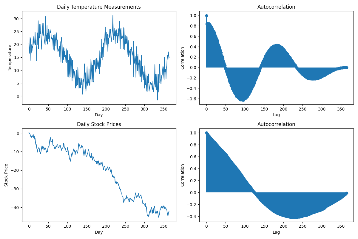
For example, consider the temperature measurements taken every day for a year. There is likely to be a high degree of autocorrelation because the temperature on a given day is likely to be similar to the temperature on the previous day, due to the cyclical nature of seasons. In contrast, the daily stock prices of a company may have lower autocorrelation, as they are influenced by many factors and can change rapidly from day to day.
Autocorrelation is an essential concept in time series analysis, as it can help to identify repeating patterns, inform modeling choices, and diagnose potential issues such as autocorrelated errors in regression models.
Definition
Autocorrelation can be represented mathematically by a function called the autocorrelation function (ACF). The ACF takes into account the time lag (the number of time steps separating two data points) and computes the correlation coefficient for each lag. The resulting plot can provide insights into the underlying structure and dependencies within the time series data.
A positive autocorrelation means that the values of the time series tend to follow the same direction (increasing or decreasing) at different time lags, while a negative autocorrelation indicates that the values tend to change direction (increase after a decrease or vice versa). If there's no autocorrelation, the time series is considered to be random or independent.
We'll start with the definition of the covariance between two variables and then define the autocorrelation function (ACF).
Covariance is a measure of how two variables change together. For two random variables \(X\) and \(Y\) with mean values \(μ_X\) and \(μ_Y\), the covariance is given by:
\[ \text{Cov}(X, Y) = \mathbb{E}[(X - \mu_X)(Y - \mu_Y)] \]
Now, let's focus on autocorrelation. Consider a discrete-time series, \(x(t)\), where \(t = 1, 2, 3, ... , N\). The mean value of the time series is given by:
\[ \mu_x = \frac{1}{N} \sum_{t=1}^{N} x(t) \]
For a given time lag \(k\), the autocovariance between \(x(t)\) and \(x(t+k)\) is defined as:
\[
\gamma(k) = \mathbb{E}[(x(t) - \mu_x)(x(t+k) - \mu_x)] \quad \text{for} \quad t = 1 \text{ to } N-k,
\]
where \(γ(k)\) represents the autocovariance at lag \(k\), and \(E[.]\) denotes the expected value.
The autocorrelation function (ACF), denoted as \(ρ(k)\), is obtained by normalizing the autocovariance function with respect to the variance of the time series (which is the autocovariance at lag \(0, γ(0)\)):
\[ \rho(k) = \frac{\gamma(k)}{\gamma(0)} \]
The ACF ranges from -1 to 1, with -1 indicating perfect negative autocorrelation, 1 indicating perfect positive autocorrelation, and 0 indicating no autocorrelation. By calculating \(ρ(k)\) for different values of \(k\), we can analyze the correlation structure of the time series at various lags.
These equations provide the foundation for understanding autocorrelation and working with time series data.
Here are two examples of autocorrelation. In the first one, we have a sine function of 20 Hz sampled at 1000Hz. We can observe that there are on every 50 unit lag. Intuitively, the signals should overlap on \({1000\text{Hz} \over 20\text{Hz} = 50} intervals.
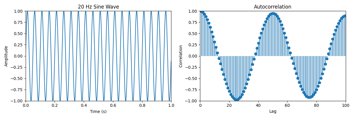
In the following, is an animation that shows more clearly how the lagged version of the signal relates to the original one.
The second example is a bit more complex. Here, we have two sine functions 20 Hz + 50 Hz sampled at 1000Hz. We can observe that there are now more peaks as the level of overlap varies significantly for more complex signals.
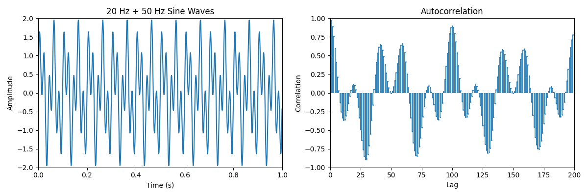
This is can be more easily observed in the following animation of the same scenario.
Intuitively, autocorrelation provides insights into the underlying patterns or trends within a time series of data that persist over time. A positive autocorrelation means that the values of the time series tend to follow the same direction (increasing or decreasing) at different time lags, while a negative autocorrelation indicates that the values tend to change direction (increase after a decrease or vice versa). If there's no autocorrelation, the time series is considered to be random or independent.
Relation between the lag and sampling rate
The sampling rate is related to the unit of lag in the autocorrelation function. The lag represents the time shift applied to the signal when comparing it to itself, and it is usually measured in discrete units, called "lag steps" or simply "lags." These discrete units correspond to the time intervals between the samples in the time series.
The relationship between the sampling rate and the unit of lag can be defined as follows:
- Time per lag unit: The time per lag unit is the inverse of the sampling rate (1/sampling rate). It represents the time interval between two consecutive samples in the time series. For example, if the sampling rate is 100 Hz (100 samples per second), the time per lag unit would be 1/100 s = 0.01 s.
- Maximum lag time: The maximum lag time that can be analyzed in a time series is determined by the duration of the signal. The longer the signal, the larger the maximum lag time that can be investigated. However, it's important to note that when the lag becomes too large, the number of overlapping points between the original and lagged signals decreases, which can lead to less reliable autocorrelation estimates.
- Lag units for a specific time shift: If you want to investigate a specific time shift in your autocorrelation analysis, you can calculate the number of lag units corresponding to that time shift using the sampling rate. To do this, simply divide the desired time shift by the time per lag unit (or multiply the time shift by the sampling rate).
For example, if you have a time series with a sampling rate of 100 Hz and you want to investigate a time shift of 0.05 seconds, you would need to use a lag of \(0.05 s \times 100 \text{samples}/s = 5 \text{lag units}\).
The sampling rate determines the unit of lag in the autocorrelation function by defining the time interval between consecutive samples. To analyze a specific time shift in the autocorrelation function, you can calculate the corresponding number of lag units based on the sampling rate.
Weak or Strong autocorrelation
Autocorrelation can be characterized as strong or weak depending on the strength of the relationship between the values in a time series and their past values.
Strong autocorrelation means that the values in the time series are highly correlated with their past values. In this case, the autocorrelation function (ACF) will show relatively high correlation coefficients for one or more lags, indicating a strong dependence on past values. Time series with strong autocorrelation often exhibit clear patterns, trends, or seasonality, making them more predictable.
Weak autocorrelation, on the other hand, means that the relationship between a variable's current value and its past values is weak or negligible. The ACF will show low correlation coefficients for most lags, suggesting that the values in the time series are relatively independent of their past values. In this case, the time series may appear more random or less predictable.
It's important to note that the strength of autocorrelation can vary between different lags. For example, a time series might exhibit strong autocorrelation at a specific lag (e.g., a 24-hour lag in hourly temperature data) but have weak autocorrelation at other lags.
Determining whether autocorrelation is strong or weak can be useful in time series analysis and forecasting. If a time series exhibits strong autocorrelation, incorporating this information into a model can lead to more accurate predictions. Conversely, if autocorrelation is weak, relying on past values may not be as beneficial for forecasting, and other techniques might be more appropriate.
Implementation of autocorrelation
In practice, autocorrelation is calculated using either the time-domain method or the frequency-domain method. The choice between the time-domain and frequency-domain methods depends on factors such as the size of the dataset, the required precision, and computational resources. For small datasets, the time-domain approach may be more straightforward. In contrast, for larger datasets, the frequency-domain method can offer computational advantages due to the efficiency of the FFT algorithm.
To see how autocorrelation can be calculated in Python, check the following article.

Time-domain method
The time-domain method involves directly calculating the autocorrelation function (ACF) for a discrete-time signal \(x[n]\) using the following formula:
\[ R[k] = \sum_{n=k}^{N-1}x[n] x[n - k],
where \(R[k]\) is the autocorrelation at lag \(k\), \(N\) is the total number of samples in the signal, and \(x[n]\) is the value of the signal at time index \(n\). Essentially, you calculate the product of the signal and its lagged version at each time step and then sum these products for all time steps within the overlapping range.
The complexity of the time-domain method is generally \(O(NM)\), where \(N\) is the number of samples and \(M\) is the maximum lag considered. While simpler to implement, for large data sets, they are computational complexity considerations.
Frequency-domain method
The frequency-domain method is based on the Wiener-Khinchin theorem, which states that the autocorrelation function of a signal is the inverse Fourier transform of the power spectral density (PSD) of the signal. This method can be more computationally efficient when dealing with large datasets, as it utilizes the Fast Fourier Transform (FFT) algorithm.
In practice, the choice between the time-domain and frequency-domain methods depends on factors such as the size of the dataset, the required precision, and computational resources. For small datasets, the time-domain approach may be more straightforward. In contrast, for larger datasets, the frequency-domain method can offer computational advantages due to the efficiency of the FFT algorithm. This algorithm has a complexity of \(O(N\log(N))\). In this case, the frequency-domain method can offer significant computational advantages for large datasets.
Computational complexity considerations
The computational complexity of autocorrelation depends not only on the method but also on several factors other factors, including the size of the dataset, the maximum lag considered, and the choice of algorithm. Here are some key parameters that affect the complexity:
Size of the dataset (N): The number of samples in the time series directly affects the computational complexity of autocorrelation. As the dataset size increases, the number of calculations required for both time-domain and frequency-domain methods increases, leading to higher computational complexity.
Maximum lag considered (M): The maximum lag considered in the ACF calculation also affects the computational complexity. As you increase the maximum lag, the number of computations in the time-domain method increases linearly, while the complexity of the frequency-domain method remains mostly unaffected, as the Fourier transform has to be calculated only once for the entire dataset.
Examples of autocorrelation
Temperature data: Daily temperature data usually exhibits strong autocorrelation because temperature changes are often gradual, and the temperature on a given day is influenced by the temperature on the previous day.
Stock prices: Stock prices might exhibit weak autocorrelation, as they are influenced by numerous factors and can be challenging to predict accurately. However, certain stock prices may exhibit some autocorrelation depending on market trends and investor behavior.
Electricity consumption: Electricity consumption often shows strong autocorrelation as it follows daily and seasonal patterns, with peaks during specific hours and higher usage during certain seasons.
Unemployment rates: Economic data like unemployment rates can exhibit autocorrelation due to the persistence of economic conditions, such as recessions or periods of growth.
River flow data: River flow data may exhibit autocorrelation, as factors like precipitation, snowmelt, and human intervention can influence river flow over multiple consecutive days or weeks.
Advanced examples of autocorrelation
Here are five more advanced examples of the use of autocorrelation involving more mathematical details
Autoregressive (AR) models: Autoregressive models are used in time series analysis and rely on the concept of autocorrelation. An AR(p) model assumes that the current value of a time series depends linearly on its previous p values plus an error term. The model can be written as:
\[
x(t) = c + \sum_{i=1}^{p} \phi_i x(t-i) + \varepsilon(t),
\]
where \(x(t)\) is the value of the time series at time \(t, c\) is a constant, \(φ_i\) are the autoregressive coefficients, and \(ε(t)\) is the error term.
Moving average (MA) models: Another time series modeling technique, the moving average model, also involves autocorrelation. An MA(q) model assumes that the current value of a time series depends linearly on the past q error terms. The model is represented as:
\[
x(t) = \mu + \varepsilon(t) + \sum_{i=1}^{q} \theta_i \varepsilon(t-i),
\]
where \(x(t)\) is the value of the time series at time \(t, μ\) is the mean of the time series, \(θ_i\) are the moving average coefficients, and \(ε(t)\) is the error term.
Partial autocorrelation function (PACF): The partial autocorrelation function is another mathematical concept related to autocorrelation. After removing the effects of correlations at shorter lags, it measures the correlation between a variable's current value and its past values at a specific lag. PACF can be used to identify the order of an autoregressive model.
Autocorrelation-based tests for randomness: Tests like the Ljung-Box test and the Durbin-Watson test use autocorrelation to determine if a time series is random or exhibits patterns. These tests calculate a statistic based on the autocorrelation function and compare it to a critical value to determine if the null hypothesis of randomness can be rejected.
Spectral analysis: Autocorrelation is connected to spectral analysis, which is a technique used to analyze the frequency components of a time series. The power spectral density (PSD) of a time series can be obtained from its autocorrelation function using the Fourier transform. Spectral analysis can help identify dominant frequencies and periodicities in the data, which can be useful for filtering or decomposing the time series into its constituent components.
These examples demonstrate how autocorrelation plays a significant role in various aspects of time series analysis and signal processing.
Conclusion
In conclusion, autocorrelation is a powerful tool for analyzing time series data by measuring the correlation between a signal and its lagged versions. It is useful for detecting patterns, trends, and seasonality in various types of data, such as temperature measurements and stock prices. There are different methods to compute autocorrelation, including the time-domain method, which directly calculates the autocorrelation function (ACF), and the frequency-domain method, which leverages the Fourier transform and the power spectral density (PSD). The choice between these methods depends on factors such as the size of the dataset and the required precision.
The computational complexity of autocorrelation is influenced by several factors, including the method used, the size of the dataset, the maximum lag considered, and the choice of algorithm. The time-domain method typically has a complexity of \(O(NM)\), while the frequency-domain method, which relies on the Fast Fourier Transform (FFT) algorithm, has a complexity of \(O(N\log N)\). The sampling rate also plays a crucial role in autocorrelation analysis, as it determines the unit of lag and affects the resolution of the ACF. By carefully selecting the appropriate method, algorithm, and sampling rate, autocorrelation can be effectively employed to uncover hidden relationships and patterns in time series data.