Python for Time Series Analysis: 4 Techniques for Autocorrelation Function Calculation

Autocorrelation is a function that provides a correlation of a data set with itself on different delays (lags). This has many applications in statistics and signal processing. This subject was touched on in our previous post on how to write a pitch detection algorithm in Python using autocorrelation. Also if you are looking for a more in-depth view of autocorrelation, see the Practical Guide to Autocorrelation.
What is autocorrelation function?
Autocorrelation, also known as serial correlation, is a statistical concept that refers to the correlation of a signal with a delayed copy of itself as a function of delay. This concept is commonly used in signal processing and time series analysis.
In a time series context, autocorrelation can be thought of as the correlation between a series and its lagged values. For example, in daily stock market returns, autocorrelation might be used to measure how today's return is related to yesterday's return.
If a series is autocorrelated, it means that the values in the series are not independent of each other. For example, if a positive autocorrelation is detected at a lag of 1, it means that high values in the series tend to be followed by high values, and low values tend to be followed by low values.
Mathematically, the autocorrelation function (ACF) is defined as the correlation between the elements of a series and others from the same series separated from them by a given interval. We can write this for real-valued discrete signals as \[R_{ff}(l) = \sum_{n=0}^N f(n)f(n - l).\] Definition for continuous and random signals can be found, e.g., from Wikipedia.

Obviously, the maximum is at lag \(l = 0\). If the peaks of the ACF occur at even intervals, we can assume that the signal periodic component at that interval.
Let's consider a 10Hz sine wave, and sample this wave with a 1000Hz sampling rate.
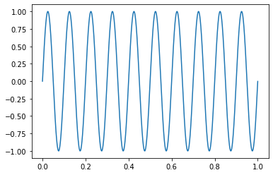
With the 1000Hz sampling rate, we will have 100 samples per full period of the wave. Now, look at the autocorrelation function on the sine wave
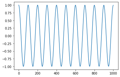
Look's almost the same. Notice how we have a maximum at \(l = 0\). Since our signal is perfectly periodic, we will have a maximum at each period. That's every 100 samples or \(l = 100\).
In our following implementations, we consider the ACF, where we normalize the range between \([1, -1]\). This output comparison is easier. There are different varieties depending on the application and somewhat on the definition.
The degree of correlation determined by correlation coefficients
- A correlation coefficient close to 1 indicates a strong positive autocorrelation. That is, a high value in the time series is likely to be followed by another high value, and a low value is likely to be followed by another low value.
- A correlation coefficient close to -1 indicates a strong negative autocorrelation. That is, a high value in the time series is likely to be followed by a low value, and vice versa.
- A correlation coefficient closer to 0 indicates no correlation. That is, the values in the time series appear to be random and do not follow a discernible pattern.
Data set and number of lags to calculate
Before going into the methods of calculating autocorrelation, we need to have some data. You can find below the data set that we are considering in our examples. The data consists of a list of random integers. It could be anything really, but here we did not want to provide the data any specific properties. Thus, we made it random.
In addition to a data set, we need to know how many lag points we are interested in calculating. In this case, we've chosen 10 points. We could have calculated the autocorrelation of all possible lags (the same as data set length). However, for some of the methods shown here, the computational complexity is relative to the number of lags. We want to highlight this by choosing only a subset of lags to consider.
# Our data set
data = [3, 16, 156, 47, 246, 176, 233, 140, 130,
        101, 166, 201, 200, 116, 118, 247,
        209, 52, 153, 232, 128, 27, 192, 168, 208,
        187, 228, 86, 30, 151, 18, 254,
        76, 112, 67, 244, 179, 150, 89, 49, 83, 147, 90,
        33, 6, 158, 80, 35, 186, 127]

# Delay (lag) range that we are interesting in
lags = range(10)
4 Ways of Calculating Autocorrelation
Now, to the point. Here are four different ways of implementing the ACF. One is a vanilla Python implementation without any external dependencies. The other three use common statistics/mathematics libraries.
Python only
This is a Python-only method without any external dependencies for calculating the autocorrelation.
''' Python only implementation '''

# Pre-allocate autocorrelation table
acorr = len(lags) * [0]

# Mean
mean = sum(data) / len(data)

# Variance
var = sum([(x - mean)**2 for x in data]) / len(data)

# Normalized data
ndata = [x - mean for x in data]


# Go through lag components one-by-one
for l in lags:
    c = 1 # Self correlation

    if (l > 0):
        tmp = [ndata[l:][i] * ndata[:-l][i]
               for i in range(len(data) - l)]

        c = sum(tmp) / len(data) / var

    acorr[l] = c
Output with our test data set
[ 1. , 0.07326561, 0.01341434, -0.03866088, 0.13064865,
  -0.05907283, -0.00449197,  0.08829021, -0.05690311,
  0.03172606]
Statsmodels library
Statsmodels is a great library for statistics and it provides a simple interface for computing the autocorrelation. This is the simplest one to use. You just give the data and how many lag points you need.
''' Statsmodels '''

import statsmodels.api as sm

acorr = sm.tsa.acf(data, nlags = len(lags)-1)
Output with our test data set
[ 1. , 0.07326561, 0.01341434, -0.03866088, 0.13064865,
  -0.05907283, -0.00449197, 0.08829021, -0.05690311,
  0.03172606]
Numpy.correlate
Numpy provides a simple function for calculating correlation. Since autocorrelation is basically correlation for a data set with itself, it is no surprise that there is a way to use numpy.correlate to calculate autocorrelation.
''' numpy.correlate '''

import numpy

x = np.array(data)

# Mean
mean = numpy.mean(data)

# Variance
var = numpy.var(data)

# Normalized data
ndata = data - mean

acorr = numpy.correlate(ndata, ndata, 'full')[len(ndata)-1:]
acorr = acorr / var / len(ndata)
Output with our test data set
[ 1. , 0.07326561, 0.01341434, -0.03866088, 0.13064865,
  -0.05907283, -0.00449197,  0.08829021, -0.05690311,
  0.03172606]
Fourier Transform
It turns out that autocorrelation is the real part of the inverse Fourier transform of the power spectrum. This follows from the Wiener–Khinchin theorem. We can exploit this, and write the following simple algorithm
- Take the Fourier transform of our data set.
- Calculate the corresponding power spectrum.
- Take the inverse Fourier transform of the power spectrum and you get the autocorrelation.
''' Fourier transform implementation '''

import numpy

# Nearest size with power of 2
size = 2 ** numpy.ceil(numpy.log2(2*len(data) - 1)).astype('int')

# Variance
var = numpy.var(data)

# Normalized data
ndata = data - numpy.mean(data)

# Compute the FFT
fft = numpy.fft.fft(ndata, size)

# Get the power spectrum
pwr = np.abs(fft) ** 2

# Calculate the autocorrelation from inverse FFT of the power spectrum
acorr = numpy.fft.ifft(pwr).real / var / len(data)
Output with our test data set
[ 1. , 0.07326561, 0.01341434, -0.03866088, 0.13064865,
  -0.05907283, -0.00449197, 0.08829021, -0.05690311,
  0.03172606]
Durbin-Watson test
The Durbin-Watson test is a statistical test used to check for autocorrelation in the residuals from a statistical regression analysis. Specifically, it's often used to detect ACF at lag 1. It's named after statisticians James Durbin and Geoffrey Watson.
The test statistic is approximately equal to 2*(1-r), where r is the sample ACF of the residuals. Therefore, for r == 0, indicating no autocorrelation, the test statistic equals 2. The statistic ranges from 0 to 4, and a value close to 2 suggests there is no autocorrelation. If the statistic is significantly less than 2, there is evidence of positive autocorrelation, and if it's greater than 2, it suggests negative autocorrelation.
In Python, you can use the Durbin-Watson test through the statsmodels package. Here is a basic example:
import statsmodels.api as sm
import statsmodels.formula.api as smf

# load a sample dataset
data = sm.datasets.get_rdataset('mtcars').data

# fit a linear regression model
model = smf.ols('mpg ~ cyl + disp + hp', data=data).fit()

# calculate Durbin-Watson statistic
dw = sm.stats.durbin_watson(model.resid)

print('Durbin-Watson statistic:', dw)
In this example, we load the mtcars dataset from statsmodels, fit a linear regression model, and then calculate the Durbin-Watson statistic on the residuals of the model. The Durbin-Watson statistic is a single number that you can interpret as described above.
As with any statistical test, you should interpret the Durbin-Watson statistic in the context of your specific analysis and data. The Durbin-Watson test is just one tool to detect autocorrelation, and it might not be appropriate for all cases. For instance, it is most powerful for detecting first-order autocorrelation and may not be as effective at identifying higher-order autocorrelation.
Summary
As expected, all four methods produce the same output. It is up to you, which approach is the most convenient for you. The performance difference is out of the scope of this post, but as your data set starts to increase in size you can expect an exponential increase in complexity.