Pitch detection using Python and autocorrelation
Pitch detection algorithm in python. Using autocorrelation as the dominant frequency detection tool.

Pitch detection can be useful in many situations. There are many ways of doing it. Here we'll investigate a simple one that uses autocorrelation to detect the dominant pitch from an audio sample. While this approach may not be the most robust one, it's straightforward to implement and a fun example of how to use autocorrelation.
Autocorrelation - the basic theory
Autocorrelation, in simple terms, is the correlation of a signal with itself on different delays. We can write this for real-valued discrete signals as \[R_{ff}(l) = \sum_{n=0}^N f(n)f(n - l).\] Definition for continuous and random signals can be found, e.g., from Wikipedia.

Obviously, the maximum is at lag \(l = 0\). If the peaks of the autocorrelation function occur at even intervals, we can assume that the signal periodic component at that interval.
Let's consider a 10Hz sine wave, and sample this wave with a 1000Hz sampling rate.
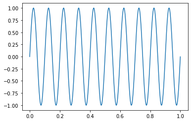
With the 1000Hz sampling rate, we will have 100 samples per full period of the wave. Now, look at the autocorrelation function on the sine wave
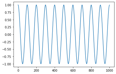
Look's almost the same. Notice how we have a maximum at \(l = 0\). Since our signal is perfectly periodic, we will have a maximum at each period. That's every 100 samples or \(l = 100\).
For our pitch detection algorithm, we would like to be able to pick up the frequency of the signal from the autocorrelation. If we know the sampling frequency (\(s = 1000\text{Hz}\)), we can pick the frequency corresponding to the lag as \[f = {s \over l} = {1000\text{Hz} \over 100} = 10\text{Hz}.\]
For a more in-depth view of autocorrelation, see the Practical Guide to Autocorrelation
The trivial pitch detection algorithm
The algorithm is pretty straightforward. Following the discussion above, we have the steps to implement a pitch detection algorithm
- Determine the sampling rate (\(s\)) for the signal
- Compute the autocorrelation for the signal
- Find peak lag (\(l\)) from the autocorrelation \(l > 0\).
- Compute the corresponding pitch frequency for the peak lag \[f = {s \over l}.\]
Python implementation
We use Tuning fork 1 from the Soundboard as our data set. It has a recording of 440Hz tuning fork.
We begin with the usual import preamble. librosa is used to load the mp3 data set and statsmodels provides us the autocorrelation. scipy.signals gives us the peak detection algorithm.
import librosa
import matplotlib.pyplot as plt
import numpy as np
import statsmodels.api as sm
from scipy.signal import find_peaks
Loading the data set is simple as `librosa` takes care of all the details.
# Load data and sampling frequency from the data file
data, sampling_frequency = librosa.load('./Tuning fork 1.mp3')

# Get some useful statistics
T = 1/sampling_frequency # Sampling period
N = len(data) # Signal length in samples
t = N / sampling_frequency # Signal length in seconds
Computing the spectrum is optional. We use it to verify our results.
Y_k = np.fft.fft(data)[0:int(N/2)]/N # FFT
Y_k[1:] = 2*Y_k[1:] # Single-sided spectrum
Pxx = np.abs(Y_k) # Power spectrum

f = sampling_frequency * np.arange((N/2)) / N; # frequencies

# plotting
fig,ax = plt.subplots()
plt.plot(f[0:5000], Pxx[0:5000], linewidth=2)
plt.ylabel('Amplitude')
plt.xlabel('Frequency [Hz]')
plt.show()
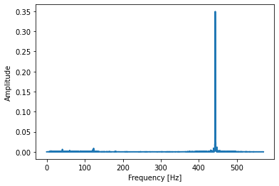
The spectrum clearly shows that we have a dominant frequency at 440-450 Hz. This is what we should be looking for also from the autocorrelation.
Use statsmodels acf function to compute the autocorrelation. We limit the number of lags to compute to 2000. This is because we have a rough idea for the range of the pitch.
auto = sm.tsa.acf(data, nlags=2000)
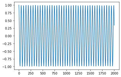
From the autocorrelation function, it is fairly obvious that there is a strong periodic component in the signal.
Next, we use the peak detection algorithm to find the peak in the autocorrelation function. This will correspond to the pitch lag.
peaks = find_peaks(auto)[0] # Find peaks of the autocorrelation
lag = peaks[0] # Choose the first peak as our pitch component lag
Finally, we transform the peak lag to the corresponding frequency.
pitch = sampling_frequency / lag # Transform lag into frequency
This will give us a pitch frequency of 450 Hz, which is quite close to what we observed in the spectrum.
Further reading
Check our 4 ways of calculating autocorrelation in Python for alternatives to the statsmodels library.