Python

Diving Deep into K-Means Clustering: A Scikit-Learn Guide

Jake @Scicoding

Jun 6, 2023 • 9 min read

K-Means Clustering is a highly sought-after machine learning algorithm, celebrated for its simplicity and efficacy, and is primarily used in unsupervised learning tasks. As a partitioning technique, K-Means serves to dissect a dataset into 'K' unique, non-overlapping clusters or subgroups. Unlike supervised learning techniques that rely on pre-known labels, unsupervised learning, such as clustering, focuses on finding inherent structure in the data, where the exact outcome isn't known in advance.

The 'K' in K-Means represents the number of clusters. This is an input parameter that the user must provide, making the task a bit challenging since the optimal number of clusters is often not known ahead of time. The goal is to assign each data point in the dataset to one of these 'K' clusters. Data points are assigned to the cluster whose mean (centroid) is nearest to them. This process aims to minimize the intra-cluster variance while maximizing the inter-cluster variance, thus creating distinct and coherent clusters. Let's break down the theory and intuition behind the K-Means Clustering method to better understand how this fascinating algorithm operates.

Unraveling the Foundations: The Theoretical Principles Behind K-Means Clustering

The objective of K-Means is straightforward: partition a dataset into 'K' distinct, non-overlapping subgroups (clusters) where each data point belongs to the cluster with the nearest mean. Here, 'K' represents the number of clusters, a parameter the user must specify.

The intuition

K-Means clustering, at its core, is a method of identifying structure within data when we don't have a clear idea of what that structure might look like. It's an exploratory technique, one that exposes the underlying patterns by partitioning the data into groups, or 'clusters'.

To understand the intuition behind K-Means clustering, we need to grapple with its objective. The goal of K-Means is to group similar data points together and segregate dissimilar ones, thereby forming clusters. But how does it define similarity? Well, it leverages the concept of distance in a multi-dimensional space, where each dimension represents a feature in the dataset. The idea is straightforward - data points that are closer in this feature space are more similar to each other than those that are farther apart.

Let's take an analogy. Suppose you have a large pile of different fruits mixed together, and you're asked to segregate them. Without knowing their exact types (labels), you might instinctively start grouping them based on characteristics like shape, size, or color. K-Means works in a somewhat similar way. Given a dataset without any labels, it starts creating groups based on feature similarities.

The 'K' in K-Means represents the number of these groups that you want the algorithm to form. The 'means' refers to the average, representing the center point (or centroid) of each group. These centroids are key to the operation of the K-Means algorithm, as they act as the 'magnets' attracting data points towards them.

To start, the algorithm initializes 'K' centroids randomly. Then, it iteratively performs two steps until convergence. First, each data point is assigned to the closest centroid, forming K clusters. Then, each centroid is updated to be the mean of all data points assigned to its cluster.

In each iteration, the clusters become more defined and the centroids shift, leading to a better representation of the inherent groups in the data. The iterations continue until the centroids no longer move significantly, indicating that the clusters have stabilized.

In essence, K-Means strives to ensure that the intra-cluster distances (distances between points within the same cluster) are minimized, and the inter-cluster distances (distances between points from different clusters) are maximized. This way, it forms distinct and homogenous clusters, thus revealing the inherent structure within the data.

The algorithm

When delving deeper into the K-Means algorithm, it is crucial to appreciate the mathematics that governs its operation. The algorithm is an iterative procedure that consists of two primary steps: assignment and update.

1 - Assignment Step

During this step, each data point is assigned to the nearest centroid. "Nearest" here is defined using a distance metric, often Euclidean distance, although other metrics can be used depending on the problem context. The Euclidean distance between a data point \(x_{ij}\) and a centroid \(\mu_i\) in a 2-dimensional space is calculated as:

\[ d(x_{ij}, \mu_i) = \sqrt{(x_{ij1}-\mu_{i1})^2 + (x_{ij2}-\mu_{i2})^2} \]

where \(x_{ij1}\) and \(x_{ij2}\) are the coordinates of the data point, and \(\mu_{i1}\) and \(\mu_{i2}\) are the coordinates of the centroid.

2 - Update Step

After each assignment, the centroid's position is updated to reflect the new mean of all data points assigned to that cluster. The new position \(\mu'_i\) of the centroid is calculated as:

\[ \mu'_i = \frac{1}{N_i} \sum_{j=1}^{N_i} x_{ij} \]

where \(N_i\) is the number of data points in cluster \(i\).

These two steps are repeated until the algorithm converges. The convergence criterion is usually that the centroids do not move significantly between iterations, or that the assignments no longer change.

This iterative procedure aims to minimize the within-cluster sum of squares (WCSS), effectively making the data points as close as possible to the centroid of their assigned cluster. The WCSS is given by:

\[ \sum_{i=1}^k \sum_{j=1}^{n}(x_{ij} - \mu_i)^2 \]

This iterative process ensures that the algorithm converges to a solution where the WCSS cannot be decreased further by changing the assignment of any data points. It's important to note that K-Means can converge to local minima, and the final solution can depend on the initial placement of centroids. Hence, it is common to run the algorithm multiple times with different initializations and choose the solution with the lowest WCSS.

K-Means Clustering with Scikit-Learn

Scikit-Learn is a simple and efficient tool for predictive data analysis. It is built on NumPy, SciPy, and matplotlib, making it a robust tool that can easily integrate with other Python libraries.

Let's walk through a basic implementation of K-Means Clustering using Scikit-Learn:

First, we import the necessary libraries:

from sklearn.cluster import KMeans
import numpy as np
import matplotlib.pyplot as plt

Import sklearn, numpy and matplotlib

Let's generate some artificial data for clustering:

from sklearn.datasets import make_blobs
X, y = make_blobs(n_samples=300, centers=4, cluster_std=0.60, random_state=0)

Creating the example dataset

To perform K-Means clustering using Scikit-Learn, we first initialize the KMeans class:

kmeans = KMeans(n_clusters=4)

Initialize the algorithm for 4 clusters

Then, we fit our data into the model using the .fit() method:

kmeans.fit(X)

Calculate the means

Now, we can retrieve the labels and cluster centers:

labels = kmeans.labels_
centers = kmeans.cluster_centers_

Get the labels and centers

And finally, plot the clusters:

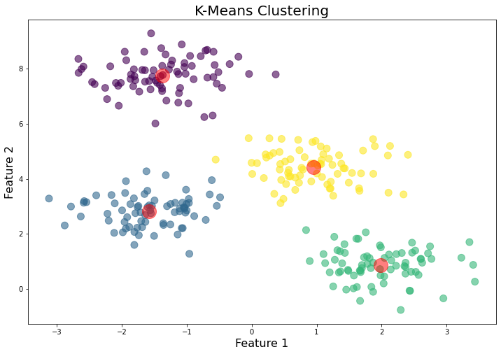
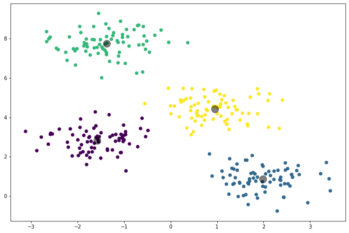
plt.scatter(X[:,0], X[:,1], c=labels, cmap='viridis')
plt.scatter(centers[:,0], centers[:,1], c='black', s=200, alpha=0.5)
plt.show()

Plot the results

This will visualize the data points colored by their cluster assignment and the cluster centers are marked in black.

Key Features of Scikit-Learn's K-Means

Scalability: Scikit-Learn's implementation of K-Means is highly scalable. It uses the K-Means++ initialization scheme by default, which gives a smarter starting point and can result in faster convergence. Moreover, it also uses the Elkan variation of the K-Means algorithm for better efficiency on lower dimensional data.

Preprocessing: The K-Means algorithm is sensitive to the scales of the data. Therefore, it's often a good idea to rescale your data before feeding it to the algorithm. Scikit-Learn provides the StandardScaler class for this purpose.

Evaluation Metrics: Scikit-Learn provides several metrics to evaluate the quality of the clustering, such as inertia (sum of squared distances to the closest centroid for each sample) and silhouette score (a measure of how close each sample in one cluster is to the samples in the neighboring clusters).

Flexibility: Scikit-Learn's K-Means can work well with various types of data and can be integrated into a larger machine-learning pipeline, taking advantage of Scikit-Learn's full suite of preprocessing methods and metrics.

In summary, the KMeans class in Scikit-Learn provides a powerful and flexible tool for performing K-Means clustering on a dataset. With its advanced features and easy-to-use interface, it allows practitioners to apply this algorithm effectively across a variety of domains and use cases.

The Choice of K

The choice of k in K-Means, which represents the number of clusters, is a critical factor that determines the effectiveness of the clustering process. However, in practice, the optimal number of clusters is not known ahead of time, as K-Means is an unsupervised method, typically used when class labels are unknown. Therefore, finding a suitable k becomes a fundamental task.

There are several methods that can help in identifying the right number of clusters:

1. The Elbow Method: This method involves running the K-Means algorithm multiple times over a loop, with an increasing number of cluster choice and then plotting a clustering score as a function of the number of clusters. The score could be the inertia (sum of squared distances to the closest centroid for all observations) or any other metric that represents the compactness of the clusters. The idea is that as we increase the number of clusters, the score improves and the rate of improvement becomes rapidly smaller at a certain point. This point is like an "elbow" in the plot, and this number of clusters is chosen.

Here's a small code snippet using the Elbow method:

from sklearn.cluster import KMeans
import matplotlib.pyplot as plt

# Some generated or real data
# X = np.array([...])

inertias = []
for i in range(1, 11):
    kmeans = KMeans(n_clusters=i, init='k-means++', max_iter=300, n_init=10, random_state=0)
    kmeans.fit(X)
    inertias.append(kmeans.inertia_)
    
plt.plot(range(1, 11), inertias)
plt.title('The Elbow Method')
plt.xlabel('Number of clusters')
plt.ylabel('Inertia')
plt.show()

Elbow method using sklearn

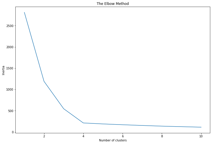
In the resulting plot, the "elbow" point represents a good choice for k.

2. The Silhouette Method: This method provides a graphical tool to determine the number of clusters. For each sample, the Silhouette Coefficient is calculated using the mean intra-cluster distance and the mean nearest-cluster distance. It's a measure of how similar an object is to its own cluster compared to other clusters. Silhouette Coefficients near +1 indicate that the sample is far away from the neighboring clusters. A negative value indicates that the sample might have been assigned to the wrong cluster.

from sklearn.metrics import silhouette_score

silhouette_scores = []
for i in range(2, 11):
    kmeans = KMeans(n_clusters=i, init='k-means++', max_iter=300, n_init=10, random_state=0)
    kmeans.fit(X)
    score = silhouette_score(X, kmeans.labels_)
    silhouette_scores.append(score)

plt.plot(range(2, 11), silhouette_scores)
plt.title('The Silhouette Method')
plt.xlabel('Number of clusters')
plt.ylabel('Silhouette Score')
plt.show()

Silhuette method using sklearn

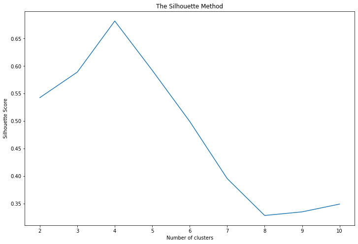
In the plot of Silhouette Score versus the number of clusters, the optimal k is the one that maximizes the score.

3. Gap Statistic: The Gap Statistic compares the total intracluster variation for different values of k with their expected values under the null reference distribution of the data. The estimate of the optimal clusters will be the value that maximizes the Gap Statistic.

While Scikit-Learn doesn't directly provide a way to compute the Gap Statistic, it can be computed manually by generating reference datasets and comparing them to the clustering results of the real data.

In conclusion, finding the appropriate k is more of an art than a science and can often involve a combination of the above methods along with domain knowledge. It's a crucial step in a K-Means.

Conclusion

K-Means clustering is a powerful and intuitive algorithm for partitioning data into distinct groups or clusters. By minimizing within-cluster variance and maximizing between-cluster variance, K-Means provides a means to uncover hidden patterns and structures within datasets. This algorithm's utility is evident across numerous fields, including but not limited to, market segmentation, document clustering, image segmentation, and anomaly detection.

However, it's important to note that the quality of the results provided by K-Means is heavily dependent on the proper choice of the number of clusters k and the initial placement of centroids. Techniques like the Elbow method, the Silhouette method, and the Gap Statistic can help in choosing a suitable k. Further, it's crucial to keep in mind that K-Means can be sensitive to the scale of the data and is more suitable for spherical clusters. Preprocessing techniques such as scaling the data can often be necessary to obtain optimal clustering results. Despite these considerations, K-Means remains one of the most widely used clustering algorithms due to its simplicity, efficiency, and versatility. In the era of ever-growing data, such unsupervised learning techniques continue to hold immense potential in extracting valuable insights from unexplored data.