How to Use Scikit-Learn for Principal Component Analysis (PCA)

If you're exploring data science, machine learning, or are already seasoned in these fields, you've likely come across Principal Component Analysis (PCA). It's a powerful statistical method that exposes fundamental structure of data in a way that best explains its variance. Put in more simple terms, PCA reduces the dimensionality of a dataset, while preserving as much 'useful' information as possible.

In this article, we will guide you through the process of conducting PCA using Scikit-learn, one of the most widely used Python libraries for machine learning. Scikit-learn (also known as sklearn) offers a broad array of tools, including PCA, and is built upon the core Python scientific libraries (NumPy, SciPy, and matplotlib), making it a powerful tool to have in your data science toolkit.

Why PCA?

Let's take a quick moment to understand why PCA is so valuable. Real-world data often has many features, which can lead to issues like overfitting and increased computational costs. PCA helps address these by transforming the original features into a new set of features, called principal components. These components are orthogonal (uncorrelated), enabling the model to focus on the features that contain the most information.

PCA interfaces from sklearn

Scikit-learn (sklearn) provides robust functionality for implementing PCA through its decomposition module. Here are some key functionalities:

Standard PCA: This is the basic form of PCA where the transformation is linear. It is implemented in sklearn as PCA().

Incremental PCA: For datasets that are too large to fit into memory, Incremental PCA (IncrementalPCA()) allows for partial computations. It is useful for online learning scenarios.

Kernel PCA: This is a form of PCA that uses a kernel function to project data into a higher dimensional space, making it possible to perform nonlinear dimensionality reduction. It is implemented as KernelPCA().

Sparse PCA: This variation of PCA (SparsePCA() and MiniBatchSparsePCA()) introduces sparsity into the transformed components, leading to components with a few non-zero features. This can help in interpretability.

Truncated Singular Value Decomposition (SVD): This is similar to PCA, but unlike PCA, it works on the data matrix directly instead of the covariance matrix. It's beneficial when the data matrix is sparse. It is implemented as TruncatedSVD().

PCA and Randomized PCA: Randomized PCA (PCA(svd_solver='randomized')) uses a non-deterministic method to quickly approximate the first few principal components in very high-dimensional data. It has a computation time complexity lower than standard PCA, making it useful for large datasets.

All PCA classes in sklearn come with methods to compute the explained variance ratio, singular values, inverse transformation, and to save and load PCA models.

Remember, different PCA techniques are suitable for different types of data and different problem requirements, so the choice of PCA method depends on the specific needs of your analysis or model.

Standard PCA using sklearn

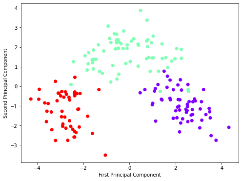
Here, is an example, which demonstrates how to use Principal Component Analysis (PCA) in sklearn to reduce the dimensionality of the Wine dataset. After loading and standardizing the dataset, PCA is performed to transform the original 13-dimensional data into 2-dimensional data, making it easier to visualize and process. The reduced data is then plotted, providing a clear visual representation of the dataset in terms of the first two principal components.

The example also illustrates how to view the explained variance ratio, offering insight into how much of the original data's variance each principal component captures. This step is key in understanding the effectiveness of PCA in preserving the 'information' from the original high-dimensional dataset during the reduction process.

Step 1: Import Required Libraries

Before we start, ensure you have the necessary libraries installed. If not, you can install them using pip:

pip install numpy
pip install sklearn
pip install matplotlib

Now, let's import the necessary libraries:

import numpy as np
from sklearn.decomposition import PCA
import matplotlib.pyplot as plt
from sklearn.preprocessing import StandardScaler
from sklearn.datasets import load_wine

Step 2: Load and Standardize the Dataset

For this article, we will use the Wine dataset, a classic dataset in the field of machine learning. It's included in sklearn's datasets module.

data = load_wine()
X = data.data
y = data.target

Before we proceed with PCA, it is important to standardize our feature set. PCA is sensitive to the variances of the initial variables. That's why the range of all features should be normalized so that each feature contributes approximately proportionately to the final distance.

scaler = StandardScaler()
X = scaler.fit_transform(X)

Step 3: Perform PCA using sklearn

Now that we have our data ready, let's perform PCA. For this example, we'll reduce the data to two dimensions.

pca = PCA(n_components=2)
X_pca = pca.fit_transform(X)

The fit_transform() function fits the PCA model with the data, and then it applies the dimensionality reduction on the data.

Step 4: Visualize the Results

It's always helpful to visualize the results. Here's how you can do it:

plt.figure(figsize=(8,6))
plt.scatter(X_pca[:,0], X_pca[:,1], c=y, cmap='rainbow')
plt.xlabel('First Principal Component')
plt.ylabel('Second Principal Component')
plt.show()

This will display a scatter plot where the axes are the first two principal components.

Step 5: Understand the Explained Variance

The explained variance tells us how much information (variance) can be attributed to each of the principal components.

print(pca.explained_variance_ratio_)

This will output ([0.36198848 0.1920749]) the amount of variance explained by each of the selected components. By this, we can know how much information is compressed into the first few principal components.

Why use explained variance as a performance metric for PCA

Explained variance in Principal Component Analysis (PCA) is a critical metric that indicates the amount of 'information' each principal component encapsulates. By projecting original data onto a lower-dimensional subspace, PCA seeks the directions where the data varies the most, forming the principal components. The explained variance reveals the proportion of total variance each component represents.

The importance of this metric lies in evaluating the effectiveness of PCA's dimensionality reduction. If a few components capture a high percentage of total variance, we can reduce the data's dimensionality without significant information loss. However, the decision on the number of components to retain shouldn't solely rely on explained variance but also on the context and specific machine learning problem at hand.

Conclusion

PCA is a powerful tool in the data science toolkit. It's useful for dimensionality reduction, visualization, noise filtering, and more. Using the Scikit-learn library, we can quickly and efficiently implement PCA with a few lines of code, making it accessible for data scientists and engineers of all levels.

The greatest strength of PCA lies in its ability to transform the data into a smaller dimensional space, making it easier for other machine learning algorithms to digest. However, keep in mind that PCA is not always appropriate for every dataset or every problem. Some data distributions may not benefit from PCA, and in certain cases, valuable data may be lost during the dimensionality reduction process.

Therefore, while PCA is undeniably a powerful tool, like all tools, its efficacy depends on the context of its use. It's always important to understand your data and your specific needs before deciding on the appropriate preprocessing or machine learning techniques.

Remember, the true power of machine learning and data science lies not in complex algorithms, but in their thoughtful application. Happy coding!

Additional Resources

For those interested in exploring further, consider these resources:

Scikit-learn User Guide: Scikit-learn's user guide is a comprehensive resource that provides detailed information about its functionalities, including PCA.

Coursera's Machine Learning Course: This course by Andrew Ng offers a deeper dive into PCA and other machine learning topics.

Python Data Science Handbook: This handbook by Jake VanderPlas provides a practical introduction to the Python data science stack, including Scikit-learn.

Now, you have a good understanding of how to use PCA using sklearn, and the world of data exploration awaits you! Keep learning, keep exploring, and keep innovating. There's no limit to what you can achieve with data science and machine learning.