Python

4 Ways to Calculate Convolution in Python

How to calculate convolution in Python. Here are the 3 most popular python packages for convolution + a pure Python implementation.

Jake @Scicoding

Aug 1, 2022 • 6 min read

Convolution is one of the fundamental operations in signal processing. Similarly to cross-correlation, it can be used to analyze the similarity of two signals with different lags.

There are many applications to convolution. It is particularly popular in image processing and machine vision, where convolution has been in edge detection and similar applications. Convolution of an input signal and impulse response gives the output of a linear time-invariant system. This makes it a very common operation in electrical engineering.

Below you can see an illustration of the convolution between square and triangular pulses.

0:00

Convolution between square and triangular pulses

In the previous posts, we have also gone through related operations and their implementations in Python:

We will have a look at three packages for calculating convolution in Python + a pure Python implementation without any dependencies.

Convolution the definition

Convolution is defined as the integral of the product of two signals (functions), where one of the signals is reversed in time. It is closely related to cross-correlation. In fact, it is cross-correlation after one of the signals has been reversed.

The definition is quite simple, you overlap the two signals with a given delay and correlate with the latter signal in reverse order. That is, one of the signals is reversed. We can write this for real-valued discrete signals as

\[R_{fg}(l) = \sum_{n=0}^N f(n)g(n - l)\]

In the following, you can see a simple animation highlighting the process. Notice how the triangle function is flipped before taking the cross-correlation, in the beginning, to reverse the input signal and perform convolution.

Definitions for complex, continuous, and random signals can be found, e.g., in Wikipedia.

Data set and number of lags to calculate

Before going into the methods of calculating convolution, we need to have some data. We use two signals as our data sets. The first one is a square pulse and the second one is a triangular pulse.

def sig_square(x):
  return 0 if x < 3 or x > 5 else 2

def sig_triag(x):
  return 0 if x < 0 or x > 2 else x

# First signal (square pulse)
sig1 = [sig_square(x/100) for x in range(1000)]

# Seconds signal (triangle pulse)
sig2 = [sig_triag(x/100) for x in range(200)]

For the sake of simplicity, we consider a one-dimensional data set. All of the considered packages also work with 2D data. This provides an obvious application for image processing.

Convolution: 3 essential packages + pure python implementation

Now, we are ready to dive into the different implementations of convolution. We begin with the Python-only implementation. This gives us the baseline. Then, we compare the results to 3 essential signal processing packages that provide their own implementation of convolution.

Native python implementation

This is a Python-only method without any external dependencies for calculating the cross-correlation. For the sake of simplicity, we don't consider any padding. That is, we will consider only the lags when the signals overlap fully.

''' Python only implementation '''
import matplotlib.pyplot as plt # Plotting only

# Pre-allocate correlation array
conv = (len(sig1) - len(sig2)) * [0]

# Go through lag components one-by-one
for l in range(len(conv)):
  for i in range(len(sig2)):
    conv[l] += sig1[l-i+len(sig2)] * sig2[i]

  conv[l] /= len(sig2) # Normalize

plt.plot(conv)

Taking convolution in Python

The output for the vanilla Python implementation should look like

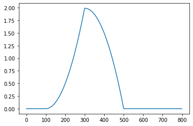
Numpy

When doing any numerical or scientific computation in Python, NumPy is usually the first package that will be imported. NumPy has a convenient implementation for convolution readily available.

You can choose the mode to handle partially overlapping signals, i.e., padding in the beginning and end of the signal. We use mode='valid', which only considers fully overlapping signals. This makes the comparison against our Python-only reference implementation easier.

''' NumPy implementation '''
import matplotlib.pyplot as plt
import numpy as np

conv = np.convolve(sig1, sig2, mode='valid')

conv /= len(sig2) # Normalize

plt.plot(conv)

Taking convolution using NumPy

The output of the NumPy implementation is identical to the Python-only implementation, which can be used to verify our implementation as well.

Check the NumPy reference manual for more examples.

Scipy

SciPy is the go-to package for numerical analysis and particularly many signal processing-specific methods. Whenever NumPy is missing the method, the SciPy should be the next target to go for.

Convolution can be found in the scipy.signal package. This method offers the same choices for padding as NumPy. In addition, you can choose between directand fft implementation. Direct implementation follows the definition of convolution similar to the pure Python implementation that we looked at before. The fft-based approach does convolution in the Fourier domain, which can be more efficient for long signals.

''' SciPy implementation '''
import matplotlib.pyplot as plt
import scipy.signal as sig

conv = sig.convolve(sig1, sig2, mode='valid')

conv /= len(sig2) # Normalize

plt.plot(conv)

The output of the SciPy implementation is identical to the Python-only and NumPy implementations.

Check the SciPy reference manual for more examples.

Astropy

Astropy is astronomy focused package and less common than the aforementioned packages. Nevertheless, it contains general-purpose functions such as convolution that are useful for other signal-processing domains as well.

Convolution in Astropy is meant to improve the SciPy implementation, particularly for scipy.ndimage. Some of these improvements include

Proper treatment of NaN values (ignoring them during convolution and replacing NaN pixels with interpolated values)
A single function for 1D, 2D, and 3D convolution
Improved options for the treatment of edges
Both direct and Fast Fourier Transform (FFT) versions
Built-in kernels that are commonly used in Astronomy

Here, we are just using the 1D convolution. These improvements are more visible when taking the higher dimension convolution.

Below, you can see how to utilize astropy.convolution to our test data. One restriction that needs to be managed is that the kernel needs to have an odd length. Thus for even signal length, we will use zero padding to make the signal non-even in length.

''' Astropy implementation '''
import matplotlib.pyplot as plt
import astropy 

# Astropy convolution requires the kernel dimensions to be odd. 
# Apply zero-padding to ensure odd dimensions
kernel = sig2
if (len(kernel) % 2 == 0):
  kernel += [0] 

conv = astropy.convolution.convolve(sig1, kernel)

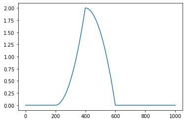
plt.plot(conv)

Taking 1D-convolution in Astropy.

Notice that we don't have explicit normalization here, as Astropy implementation has normalization on by default.

This will result in the following graph. Notice how the peak is shifted from the NumPy and SciPy versions. The shape of the convolution is identical.

Check the Astropy reference manual for more examples.

Summary

We did not compare the performance of the convolution methods. If we ignore the potential performance differences, it is pretty much a convenience-choice between the packages. Use whatever package you are using anyways. If you are after a bit more advanced features astropy might be the choice for you. Otherwise, I would go with numpy or scipy. Pure Python version should be used only for reference or if you are really trying to cut back in the dependencies, as there is very likely performance consideration.