Wireless

Water-filling algorithm implemented using Matlab & Octave

Jake

May 20, 2022 • 4 min read

In this post, I'm going to show you how to implement the water-filling algorithm using Matlab & Octave.

Matlab is a great numerical computations tool, which has been widely adopted by engineers and scientists for all sorts of numerical computations.

Water-filling is a generic method for allocating transmission power over (equalizing) communications channels in the absence of inter-channel interference (ICI). For an in-depth overview of the water-filling algorithm, check our post showing the algorithm behavior and derivation.

Basic concept

We can write the throughput for \(N\) orthogonal channels as the sum-rate over all the channels

\[ \sum_{n=1}^N \text{log}_2 (1 + \text{SNR}_n) \]

We use the sum power budget (\(P\)), which limits the available power across the channels as

\[ \sum_{n=1}^N p_n = P \]

Further, we must define the \(\text{SNR}_n\) in terms of the \(p_n\) as

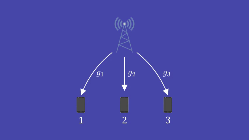
\[ \text{SNR}(p_n) = {g_n p_n \over N_0} \]

where \(g_n\) denotes the channel gain for the \(n^\text{th}\) channel, \(p_n\) is the corresponding power allocation and \(N_0\) is a fixed noise-level determined by the given SNR.

Now, we can write the capacity as

\[ C = \sum_{n=1}^N \text{log}_2 (1 + \text{SNR}(p^*_n)) \]

where \(p^*_n\) is the sum-rate maximizing power allocation for channel \(n\). Now, we have the basic premise set up to come up with an algorithm that finds the optimal power allocation, namely, the water-filling algorithm.

The algorithm

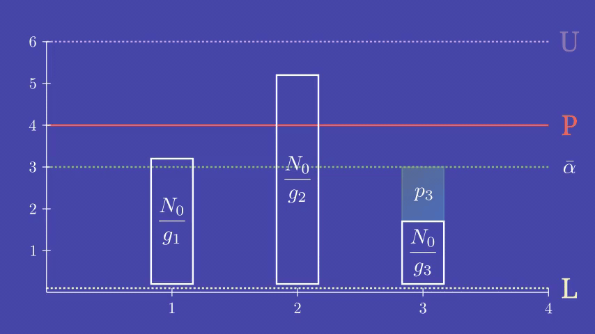
We'll skip the algorithm derivation and skip directly, our power allocation, for each channel \(n = 1,\ldots,N\), is simply given by \[ p_n = \Big({1 \over {\alpha} } - {N_0 \over g_n}\Big)^{+} \]

We can just search for such \(\alpha\) that satisfies the power budget allocation \[ \sum_{n=1}^N p_n = P \]

If you are interested in the complete derivation of the algorithm, check our previous post.

Water-filling in Matlab / Octave

Now, we are ready to jump into the implementation of the water-filling algorithm using Matlab & Octave. We avoid using any Matlab-specific functionality everything here should apply to both Matlab & Octave.

We begin, by defining the system parameters

```
% Number of channels
N = 10;
N0 = 1; % Normalized noise level
SNR_dB = 10; % Signal-to-noise ratio in dB
P = 10**(SNR_dB / 10);
```

These are the basic parameters that define the SNR ranges and the system's complexity.

Next, we need to generate channel gains for all \(N\) channels. We simply draw the from Gaussian distribution. There are more complex and realistic channel models that could be used, but those are not within the scope of this article.

% The channel specific gains drawn from Gaussian distribution
g = abs(randn(N, 1));

We start implementing the actual algorithm, by initializing the bounds for our search space. Stop threshold is used to set the point when the algorithm has converged. Our test condition is \(| \alpha_\text{low} - \alpha_\text{high} | < \epsilon_\text{stop} \)

% Bisection search for alpha
alpha_low = min(N0 / g);
alpha_high = (P + sum(N0 / g)) / N; % Initial high (upper bound)

stop_threshold = 1e-5; % Stop threshold

The complete search (bisection) loop is given by

% Iterate while low/high bounds are futher than stop_threshold
while(abs(alpha_low - alpha_high) > stop_threshold)
    alpha = (alpha_low + alpha_high) / 2; % Test value in the middle of low/high

    p = 1 / alpha - N0 / g;

    p(p < 0) = 0; % Consider only positive powers

    if (sum(p) > P)
        alpha_low = alpha;
    else
        alpha_high = alpha;
    end
end

We can see that adjusting \(\alpha\) acts as a scaling coefficient for the power allocation. Thus, increasing \(\alpha\) always lowers power allocation and vice versa. Keeping this in mind, we will implement a bisection search for the power allocation also known as the water-filling, where we search for the water level (power scaling), by bisecting the search range for \(\alpha\).

We were able to write a custom algorithm for solving the channel capacity-achieving power allocation with a couple of lines of code, just by having a look at the KKT conditions and identifying the solution. This gives us an excellent place to start for more complex systems.

The complete source can be found on Github.

Please, leave your comments and suggestions in the video comments section.

Basic concept

The algorithm

Water-filling in Matlab / Octave

Further reading