Python

Practical Guide to Random Sample Consensus (RANSAC) using Python

Jake @Scicoding

Jun 7, 2023 • 9 min read

RANSAC is a robust method for parameter estimation in the presence of outliers. It works by identifying inliers that agree with a model derived from a randomly chosen subset of data. The model with the maximum number of inliers is then chosen as the best model. In this article, we will explore the concepts behind RANSAC and its application using Python.

Brief history of RANSAC

The Random Sample Consensus (RANSAC) algorithm was introduced by Fischler and Bolles in 1981. The motivation for developing this algorithm came from the field of computer vision, where they were working on the problem of interpreting and recognizing three-dimensional scenes from two-dimensional image data.

The traditional least-squares method for fitting a model to data was often compromised by the presence of outliers in the data. Outliers could be caused by many factors including measurement errors, occlusions, or mismatches in the image correspondence problem, and these outliers had a disproportionately large effect on the estimated model. The need for a more robust method led to the development of the RANSAC algorithm.

RANSAC was a paradigm shift in the way outliers were handled. Instead of trying to mitigate the effects of outliers, it was designed to work well even in their presence. It introduced an iterative, stochastic approach to model fitting, based on the idea of consensus: a good model is one that is compatible with the largest subset of the data.

Over the years, numerous improvements and variations to the RANSAC algorithm have been proposed. Despite being over four decades old, RANSAC and its derivatives remain popular and widely used in many fields, including computer vision, robotics, geosciences, and machine learning. Its ability to handle large amounts of outliers and its general-purpose nature make it a powerful tool for robust parameter estimation.

Introduction to RANSAC

Random Sample Consensus (RANSAC) is an iterative method for robustly fitting a model to data. Its key strength is the ability to handle large amounts of outliers, making it suitable for applications in fields like computer vision, robotics, and geosciences.

RANSAC operates on the assumption that, within a dataset, there exist "inliers", data that can be explained by some model parameters, and "outliers", data that cannot be explained by the model. The algorithm works in a probabilistic manner, selecting random subsets of the original data, fitting a model to each subset, and counting inliers that fall within a certain tolerance. The model with the highest inlier count is chosen as the best model.

What are the potential applications

The Random Sample Consensus algorithm is used in a variety of fields due to its versatility and robustness against outliers. Here are a few of the many applications where RANSAC finds use:

1. Computer Vision: One of the initial applications of RANSAC was in the field of computer vision. It's extensively used for feature matching, object detection, and 3D reconstruction tasks. It's particularly useful for estimating the fundamental or essential matrix in stereo vision, the homography matrix for image stitching in panorama construction, and the camera pose in simultaneous localization and mapping (SLAM) applications.

2. Robotics: RANSAC is used in robotics for sensor data filtering and interpretation. For example, it is used in the estimation of parameters from LiDAR (Light Detection and Ranging) sensor data, where it can robustly fit models to data for tasks like plane detection and object recognition in 3D point clouds.

3. Geosciences and Remote Sensing: RANSAC is used for model fitting in geological data interpretation and also for processing and interpretation of remote sensing data. It's commonly used in applications involving the detection of structures or features in geospatial datasets, where there is often a high degree of noise and outliers.

4. Bioinformatics: In bioinformatics, RANSAC is often used in applications that involve the modeling and prediction of biological phenomena, such as gene expression levels or protein structures. It can handle the presence of experimental noise and outliers in biological datasets.

5. Machine Learning and Data Analysis: RANSAC is used to fit robust models in the presence of noisy data. In regression analysis, for example, RANSAC can provide a robust fit that is not unduly influenced by outliers.

6. Autonomous Vehicles: In autonomous driving, RANSAC is used in various sensor data processing tasks. For example, it can be used in the interpretation of radar and lidar sensor data to detect and track objects or in visual odometry to estimate the motion of the vehicle based on camera images.

7. Augmented Reality (AR): In AR, RANSAC is used to estimate the camera pose relative to a known object or pattern, enabling virtual objects to be rendered with the correct perspective and occlusions.

RANSAC is a flexible and robust method that has a wide range of applications in any field that requires fitting a model to data in the presence of outliers.

The RANSAC Algorithm

The RANSAC algorithm is an iterative method used to estimate the parameters of a mathematical model from a set of observed data that contains outliers. Its essential idea is that the correct model will be the one that is agreed upon by the maximum number of data points, hence the name "Random Sample Consensus".

Here's a more detailed breakdown of the algorithm:

Random Selection: Select a random subset of the original data of the minimum size required to fit the model. This subset is called the hypothetical inliers. For example, if we're trying to fit a line, we need at least two points. For a plane, we need at least three points.
Model Fitting: A model is fitted to the set of hypothetical inliers. This is usually done using a method that minimizes the sum of squared distances from the data points to the model, like least squares for a line or plane.
Inlier Identification: All other data are then tested against the fitted model. Those points that fit the estimated model within a predefined tolerance are considered part of the consensus set. The tolerance is usually defined in terms of distance or residual error.
Model Evaluation and Update: If the number of points in the consensus set is large enough (above a certain threshold), the estimated model is considered good. The model may then be further refined by re-estimating it using all members of the consensus set.
Iteration: This process is repeated for a predefined number of iterations. In each iteration, a new subset of data points is selected and a model is fitted to this subset. The final model chosen is the one with the largest consensus set.
Termination: The algorithm stops when either the number of iterations exceeds the predefined number, a certain computational budget has been used up, or when a model is found that fits a large enough fraction of the data.

The main parameters that control the behavior of the RANSAC algorithm are the number of iterations and the inlier tolerance. The number of iterations needed for a high probability of finding the correct model increases with the fraction of outliers in the data. The inlier tolerance, on the other hand, should be chosen based on the expected noise level in the data and the specific requirements of the task at hand.

Despite its simplicity, RANSAC is highly effective for many tasks. Its primary limitation is that it assumes that the majority of the data are inliers, which follow the model. If this assumption is violated (i.e., there are more outliers than inliers), RANSAC may fail to find the correct model.

In mathematical notation, for a dataset $D$ containing $N$ data points, the RANSAC algorithm could be summarized as:

For each iteration $i$, do:
Select a random sample $S_i$ of size $n$ from $D$.
Fit a model $M_i$ to $S_i$.
Compute the error $e_{ij}$ for each data point $j$ in $D$ relative to $M_i$.
Determine the consensus set $C_i$ containing members from $D$ that have $e_{ij}$ less than a threshold $t$.
If the size of $C_i$ is greater than a predefined threshold $T$, reestimate the model using all points in $C_i$ and terminate.
Select the model $M_k$ with the largest consensus set $C_k$.

Implementing RANSAC in Python

To illustrate RANSAC using Python, let's use a simple example: fitting a line (linear regression) to a dataset with noise and outliers. We'll use Python's popular scientific libraries: NumPy, SciPy, and Matplotlib.

Import libraries: Import the necessary packages

import numpy as np
import matplotlib.pyplot as plt
from sklearn.linear_model import LinearRegression
from sklearn.metrics import mean_squared_error

Import essential libraries

Data Generation: We are creating artificial data to demonstrate the RANSAC algorithm.

# Generating 100 inliers
X_inliers = np.linspace(-5, 5, 100)
y_inliers = 3 * X_inliers + 2 + np.random.normal(0, 0.5, 100)

# Generating 20 outliers
X_outliers = np.linspace(-5, 5, 20)
y_outliers = 30 * (np.random.random(20) - 0.5)

# Concatenating inliers and outliers into one dataset
X = np.concatenate((X_inliers, X_outliers))
y = np.concatenate((y_inliers, y_outliers))

# Reshape X for model fitting
X = X.reshape(-1, 1)

Generate test data

Here, X_inliers and y_inliers represent inlier data points that follow a line model (y = 3x + 2) with some added Gaussian noise. X_outliers and y_outliers represent outliers that are randomly distributed. We then combine these inliers and outliers to create our dataset.

Model Fitting using all data: Here, we're fitting a linear regression model to all data points, including the outliers. This model is not expected to fit well since the outliers will skew the line away from the inliers.

# Fit line using all data
model = LinearRegression()
model.fit(X, y)

# Predict y using the linear model with estimated coefficients
y_pred = model.predict(X)

Make linear prediction

RANSAC Implementation: This is where the magic happens. We begin by setting the number of iterations, the sample size, and the inlier distance threshold.

For each iteration, we do the following:

Randomly select a subset of the data of size sample_size. This forms our hypothetical inliers.
Fit a LinearRegression model to these hypothetical inliers.
Compute the residuals (the absolute differences between the observed and predicted values for all data points).
Identify the inliers as those points for which the residual is less than the threshold t.

If the number of inliers for the current model is more than any previous model, we update our best model and the maximum inlier count.

# RANSAC
n_iterations = 100
n_samples = X.shape[0]
sample_size = int(n_samples * 0.6)
t = 0.1
best_model = None
best_inlier_num = 0

for _ in range(n_iterations):
    # select random samples 
    sample = np.random.choice(n_samples, sample_size)
    X_sample = X[sample]
    y_sample = y[sample]

    # fit model to the samples
    model_sample = LinearRegression().fit(X_sample, y_sample)
    y_sample_pred = model_sample.predict(X)

    # find inliers
    residuals = np.abs(y_sample_pred - y)
    inliers = residuals < t
    inlier_num = np.count_nonzero(inliers)

    # update the best model if the current one is better
    if inlier_num > best_inlier_num:
        best_inlier_num = inlier_num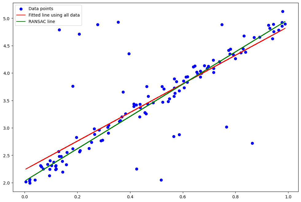
        best_model = model_sample

Make RANSAC fitting of the data

Result Plotting: Finally, we make predictions using the best model found by RANSAC and plot the data points, the line fitted using all data, and the line fitted using RANSAC. The plot shows how RANSAC provides a better fit by ignoring the outliers.

plt.figure(figsize=(12, 8))
plt.scatter(X, y, color='blue', label='Data points')
plt.plot(X, y_pred, color='red', label='Fitted line using all data'

# Plotting RANSAC's best fitted line
y_pred_ransac = best_model.predict(X)
plt.plot(X, y_pred_ransac, color='green', label='RANSAC line')
plt.legend()
plt.show()

Plot the results using Matplotlib

In this simple example, the RANSAC algorithm is used to fit a line to data points. However, the algorithm is not limited to line fitting and can be used for fitting any model to data, such as polynomials, circles, or more complex structures, as long as you can define a way to fit the model to a sample and measure how well it performs.

Implementations in other languages

Implementations of the RANSAC algorithm are available in several programming languages, often as part of larger libraries focused on computer vision, machine learning, or scientific computing. Here are a few examples:

Python: As demonstrated above, Python's Scikit-Learn library includes a RANSAC implementation in the sklearn.linear_model.RANSACRegressor class. Similarly, the OpenCV library provides RANSAC-based functions, mainly used for finding homographies or fundamental matrices in computer vision tasks.

MATLAB: MATLAB includes a function called ransac, part of the Computer Vision System Toolbox, that performs RANSAC for estimating a mathematical model.

C++: The OpenCV library in C++ also provides RANSAC-based functions. PCL (Point Cloud Library) is another robust library used for 2D/3D image and point cloud processing, which also has RANSAC and other robust estimators.

R: The ransac package in R provides a flexible interface to RANSAC.

JavaScript: Libraries such as jsfeat provide implementations of RANSAC in JavaScript.

Java: Libraries such as OpenCV's Java interface and BoofCV provide implementations of RANSAC.

Ruby: The ruby-opencv gem provides bindings to the OpenCV library, which includes a RANSAC implementation.

It's important to note that the RANSAC algorithm can also be implemented directly in any programming language. The algorithm itself is straightforward and doesn't require any language-specific features, though the implementation can be greatly simplified by using features and libraries for linear algebra, random number generation, and data manipulation.

Conclusion

RANSAC is a powerful algorithm that can robustly estimate model parameters even in the presence of a large number of outliers. It has seen successful application in a wide range of fields, and with Python's rich scientific ecosystem, applying RANSAC to your data is straightforward.

Though the code provided here uses a linear regression model for simplicity, RANSAC is not limited to linear models or even to regression. It is, in fact, a versatile method that can be used with any model that can be estimated from a sample of data, making it a valuable tool in many machine learning and computer vision tasks. Understanding and effectively implementing RANSAC can be pivotal in many data analysis and modeling situations.