Python PCA using SKLearn for Image Compression Application

Principal component analysis (PCA) provides an intuitive and analytically sound basis for various applications. Image compression is one of the most applied uses of PCA.
We are utilizing scikit-learn or sklearn for short to perform the heavy lifting in principal component analysis. No point in reinventing the wheel, by implementing PCA by ourselves. The Scikit team has done great work in providing mature and optimized PCA implementation for Python.
After reading this tutorial, you know how to apply PCA to images and extract the most information-containing components. Reducing the number of stored components can be used to compress the images. Finally, you will see how to transform the PCA components back to images, that is, you know how to decompress the images. Essentially, you have all the essential tools to build a working image compression tool utilizing principal component analysis.
Quick PCA Basics for Image Compression
Image compression is an essential technique to save storage and optimize transmission processes. When it comes to compressing high-dimensional data such as images, PCA is a robust tool for this purpose. PCA uses dimensionality reduction, which is the process of reducing the number of random variables under consideration, to retain the most significant features while cutting down the data size.
In PCA, the first step involves standardizing the original data. After standardization, the PCA algorithm is applied to fit and transform the data into a lower-dimensional space. This 'fit transform' method essentially identifies the axes or 'principal components' in the data with the most variance. These principal components represent the most substantial differences in the data, and they form the backbone of the compressed data representation.
The explained variance ratio is a fundamental concept in PCA. It tells us how much information (variance) can be attributed to each of the principal components. Usually, a few components account for most of the variance, and these are the ones we want to keep. By discarding components with low explained variance, we achieve a form of lossy compression: we throw away the least important information to reduce the data size.
Once the fit transform method is applied, the high dimensional data is compressed into a new dimensional space, typically much smaller. This process of transforming data into a lower-dimensional space not only preserves the most significant features but also aids in efficient data storage and faster data processing.
However, it's essential to note that transforming data using PCA can sometimes result in a loss of specific details. Although the principal components aim to retain as much information as possible, some original data might get lost in the compression process, which might be acceptable in many applications where a little loss of detail is tolerable compared to the benefits of reduced storage and processing requirements.
PCA-based image compression
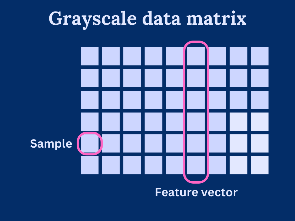
We shall start our journey to PCA and image compression considering grayscale images. Grayscale images have the benefit of having only a value to represent a pixel color, which makes the image structure more intuitive to start with. Later, we expand our methods to cover color images as well.
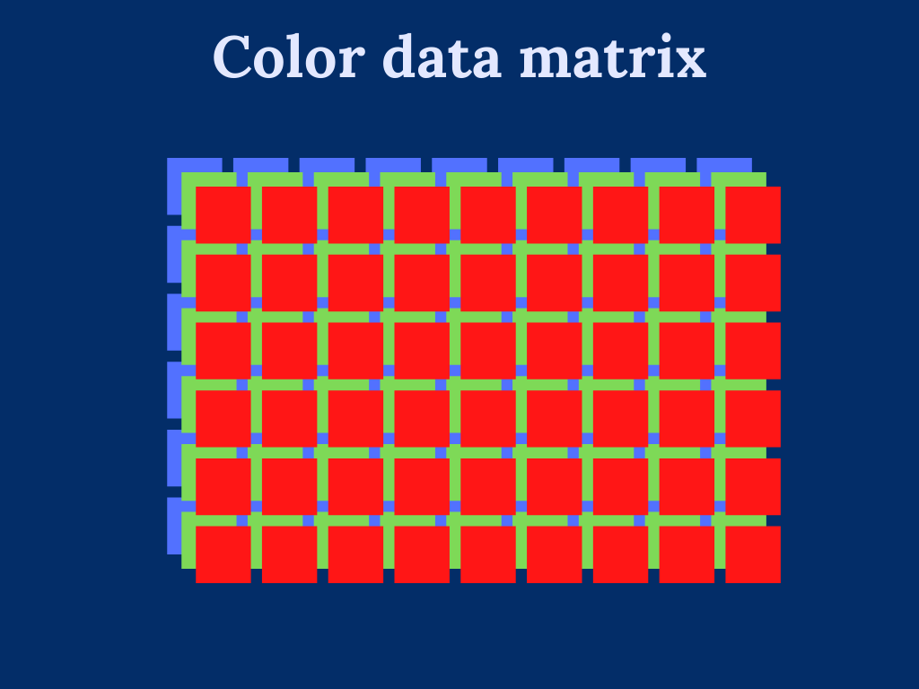
We can consider grayscale images as a data matrix or array, where each column is a feature vector and pixels are individual samples in the features. As such, the width of the image determines how many features we have and height determines the length of the feature vectors.
Generally speaking, PCA is very sensitive to feature vector scaling. That is, the vectors should cover roughly the same scale. With our image data, we can assume that the scale is similar as each element has a pixel value within [0, 255]. Of course, we could come up with images that are hard for PCA to handle, but these scenarios are out of the scope of this post.
Let's get started with an example image. This is quite a complex grayscale image. It will show quite nicely the kind of artifacts that we need to deal with when going up with the PCA compression ratio. That is, reducing the number of principal components or performing dimensionality reduction.
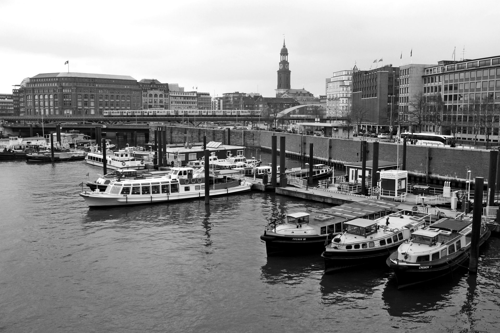
We will use the skimage (scikit-image) to load the image and convert it into a grayscale.
import skimage

path = './water.jpg'

image = skimage.io.imread(path) # Load image
image = skimage.color.rgb2gray(image) # Convert to grayscaleThe image array has shape (1280, 1920). This is now suitable as-is to be used for PCA. The array columns are used as feature vectors and pixels are considered individual samples.
Now, using the image as a data set, we can utilize sklearn.decomposition.PCA to calculate the principal components.
There are two phases to our image compression routine:
- Calculate the principal components for a given image
- Transform (project) the image into the basis of the calculated principal components
Decompression will be simply a reverse transformation of the image data.
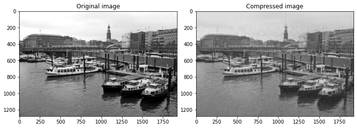
Let's dive right into it and look at the details a bit later. Let's first try to compress the image using only 50 PCA vectors
import matplotlib.pyplot as plt
from sklearn.decomposition import PCA

pca = PCA(n_components=50)
image_compressed = pca.fit_transform(image)
image_decompressed = pca.inverse_transform(image_compressed)

fig, axes = plt.subplots(1,2, figsize=(100, 100))
axes[0].imshow(image, cmap='gray')
axes[0].set_label("Original image")
axes[1].imshow(image_decompressed, cmap='gray')
axes[1].set_label("Compressed image")Not too bad. As you can see below, 50 PCAs is quite enough to preserve most of the details. Sure, much of the finer details are lost, but you can quite well see the contents of the image.
Now, we can go a bit further into the PCA. One of the key questions is of course
How many principal components do we need to efficiently compress our images?
The answer is: it depends. Different images can be compressed with different artifact levels using the same principal components. It all comes down to how much of the total variance in the image, we can take into account in our principal components.
Let's see how it works out in practice. First, we will generate 512 most significant principal components using PCA. Then, we see how much of the variance is explained by those components
from sklearn.decomposition import PCA
import matplotlib.pyplot as plt

# Calculate 1000 first principal components
pca = PCA(n_components=1000).fit(image)

# Collect the explained variance of each component
explained_variance = pca.explained_variance_ratio_

# Component indices
components = [i for i in range(0, len(explained_variance))]

# Explained variance in percents
explained_variance_percent = [100 * i for i in explained_variance]

fig = plt.figure()
ax = fig.add_subplot(1, 1, 1)
ax.set_title('Explained variance by number of components')
ax.set_ylabel('Explained variance (%)')
ax.set_xlabel('Number of PCA components')

# Cumulative sum of the explained variance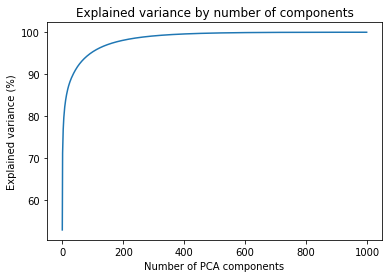
ax.plot(components, np.cumsum(explained_variance_percent)) This gives us the following figure. From here, we can identify the impact of the number of components on the expected quality
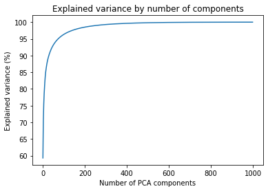
We can pinpoint a few cut-off points that we can use to test the necessary variance for good-quality images
| Components | Explained variance |
|---|---|
| 8 | 80% |
| 29 | 90% |
| 73 | 95% |
| 252 | 99% |
| 580 | 99.9% |
We should really put these numbers into some concrete examples. Let's try the out.
# Utility function that compresses image with given number
# of principal components
def compress_image(n_components, image):
    pca = PCA(n_components=n_components)
    image_compressed = pca.fit_transform(image)
    return pca.inverse_transform(image_compressed)

# Compress images with different numbers of principal components
image_8 = compress_image(8, image)
image_29 = compress_image(29, image)
image_73 = compress_image(73, image)
image_254 = compress_image(254, image)
image_580 = compress_image(580, image)

fig, axes = plt.subplots(2,3, figsize=(10,5), constrained_layout=True)

axes[0][0].imshow(image_8, cmap='gray')
axes[0][0].set_title("Compressed image (PCA: 8)")

axes[0][1].imshow(image_29, cmap='gray')
axes[0][1].set_title("Compressed image (PCA: 29)")

axes[0][2].imshow(image_73, cmap='gray')
axes[0][2].set_title("Compressed image (PCA: 73)")

axes[1][0].imshow(image_254, cmap='gray')
axes[1][0].set_title("Compressed image (PCA: 254)")

axes[1][1].imshow(image_580, cmap='gray')
axes[1][1].set_title("Compressed image (PCA: 580)")

axes[1][2].imshow(image, cmap='gray')
axes[1][2].set_title("Original image")This gives us the following comparison
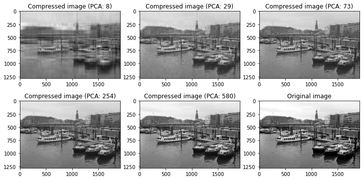
It is evident that 80% of the variance is not enough details to produce good-quality images. However, anything after 90% starts to look good, and after 95% the quality is really good.
That should give you some perspective on how much of the variance you should capture to produce a nice quality image with PCA compression.
Compression ratio
So far, we have only discussed how to perform PCA and use it to reduce the dimensionality of the image. How about the compression ratio? What is the actual data that needs to be conveyed to store and decompress the images?
Basically, we need two things:
- The principal components. That is the principal basis vectors into which we project our original image.
- We need the compressed/transformed image, which is used in the decompression phase.
The principal components, we can get from pca.components_ and the compressed image as an output for pca.fit_tranform or pca.transform.
Let's see what the compression ratio looks like.
Our original image has a size of 1280 x 1920. That is, we have 1920 column vectors of length 1280 in our original image. The length of the image columns needs to match the length of the PCA component rows. That is if we have 16 principal components, the size of pca.components_ is 16 x 1920.
On the other hand, the length of the compressed image columns matches the original image columns. Thus, for 16 components, we have the size for image_compressed to be 1280 x 16. Now, we can count the number of elements required to be stored
- PCA components: 16 x 1920 = 30720
- Compressed image: 1280 x 16 = 20480
- Total: 51200
Since the original image size was 1280 x 1920 = 2534400, our compression ratio becomes \[ {\text{Compressed elements} \over \text{Original elements} = {51200 \over 2534400} = 2\%\].
Let's now run the same analysis for our previous results, to see what kind of compression ratios, we can expect for different numbers of components
| Components | Explained variance | Compression ratio |
|---|---|---|
| 8 | 80% | 1.04% |
| 29 | 90% | 3.77% |
| 73 | 95% | 9.5% |
| 252 | 99% | 32.8% |
| 580 | 99.9% | 75.5% |
This may not be the most efficient image compression scheme. The plus side is that we don't really exploit any specific properties of the images. The same approach can be pretty much as-is applied to other forms of data also.
Working with color images

Working with color images introduces additional difficulty in dealing with multiple color channels. Essentially, we can consider multicolor images to be multiple single-color images, where each color channel defines a single image. For instance, RGB-image has three color channels: one for red color, one for green color, and one for red color.
To overcome the trouble dealing with multi-dimensional input data. We transform the color image into a two-dimensional array by stacking the color channels on top of each other.
This can be easily done by reshaping the 3-dimensional input array into two dimensions.
import skimage

path = './ship.jpg'

image_orig = skimage.io.imread(path) # Load image

width = image_orig.shape[0]
height = image_orig.shape[1]
channels = image_orig.shape[2]

image = np.reshape(image_orig, (width, height*channels))That was simple! Now, we are basically in the same situation as with the grayscale images. The only difference from the PCA point of view is that we are dealing with a bit longer feature vectors.
Moving on. Let's see how the explained variance changes when dealing with colored images. The cumulative sum of the variance follows a very similar pattern. Most of the variance is explained by ~200 components.
In the table below, we have again picked up the number of components for a few cut-off points for the explained variance. This should give us some idea of the number of components we should pick to test the compression levels.
| Components | Explained variance |
|---|---|
| 6 | 80% |
| 36 | 90% |
| 95 | 95% |
| 283 | 99% |
| 583 | 99.9% |
To plot the image compression levels, we need to make a few minor changes to the grayscale example.
- We need to reshape the images back to the original size.
- We need to convert the samples into 8-bit unsigned integer format
Otherwise, the code is pretty much the same.
# Utility function that compresses image with given number
# of principal components
def compress_image(n_components, image, size):
    pca = PCA(n_components=n_components)
    image_compressed = pca.fit_transform(image)
    return pca.inverse_transform(image_compressed).reshape(size).astype('uint8')

# Compress images with different numbers of principal components
image_6 = compress_image(6, image, image_orig.shape)
image_36 = compress_image(36, image, image_orig.shape)
image_95 = compress_image(95, image, image_orig.shape)
image_283 = compress_image(283, image, image_orig.shape)
image_583 = compress_image(583, image, image_orig.shape)

fig, axes = plt.subplots(2,3, figsize=(10,5), constrained_layout=True)

axes[0][0].imshow(image_6)
axes[0][0].set_title("Compressed image (PCA: 6)")

axes[0][1].imshow(image_36)
axes[0][1].set_title("Compressed image (PCA: 36)")

axes[0][2].imshow(image_95)
axes[0][2].set_title("Compressed image (PCA: 95)")

axes[1][0].imshow(image_283)
axes[1][0].set_title("Compressed image (PCA: 283)")

axes[1][1].imshow(image_583)
axes[1][1].set_title("Compressed image (PCA: 583)")

axes[1][2].imshow(image_orig)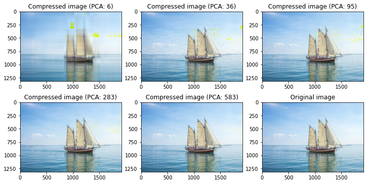
axes[1][2].set_title("Original image")The amount of detail that we can store in only a few components is quite impressive. Event with only 6 components, we can make out the outline of the image. Going up to 36 components already provides a significant amount of detail. Working with colors also introduces new types of artifacts. We can clearly see the yellow marks that are basically visible up to as high as 583 principal components. This type of color artifact is easy to spot and can be quite annoying.
The compression ratio of color images
Considering how we restructure our colors as stacked column vectors, we can the same way expand our compression ratio analysis from the grayscale images. What we will do is just consider the height of the images to be scaled by 3.
Our original image has a size of 1314 x 1920. As there are 3 color channels, we stack the columns and get the size to be (3 x 1314) x 1920 = 3942 x 1920. This means that we have 3942 x 1920 = 7568640 samples in total.
We can count the number of elements required to be stored for color images with 16 principal components to be
- PCA components: 16 x 1920 = 30720
- Compressed image: 3942 x 16 = 63072
- Total: 93792
Then, our compression ratio becomes \[ {\text{Compressed elements} \over \text{Original elements} = {93792 \over 7568640} = 1.24\%\].
Similarly, we can run the compression ratio analysis for the cutoff number of components from the previous examples.
| Components | Explained variance | Compression ratio |
|---|---|---|
| 6 | 80% | 0.46% |
| 36 | 90% | 2.79% |
| 95 | 95% | 7.35% |
| 283 | 99% | 21.9% |
| 583 | 99.9% | 45.15% |
The compression ratio is somewhat better than with the grayscale images. One factor here is of course that we used a different image. Even with the same image, it would not have been too surprising to get an improved compression ratio for the colored version as there tends to be quite a bit of redundancy between the color channels, which greatly affects the size of the "raw" uncompressed images.
Summary
You are now familiar with how to use PCA with Python to build a simple image compression framework. Working with multicolor (multichannel) images is not a problem with a few reshaping tricks you can transform them into a form that PCA accepts. You can move on to more advanced PCA topics to deepen your knowledge and fine-tune your image compression approach.