Kalman Filter with OpenCV and Python

The Kalman filter, named after its creator Rudolf E. Kalman, is a mathematical algorithm that provides recursive means to estimate the state of a system in a way that minimizes the mean squared error. It's widely used in robotics, economics, control systems, and computer vision.

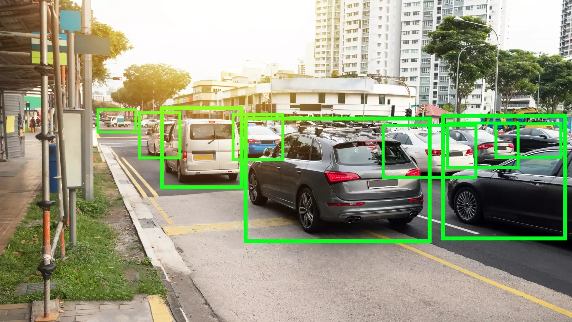
In the realm of computer vision, the Kalman filter finds extensive use in tracking applications. In this article, we'll focus on using the Kalman filter with the OpenCV library in Python, a robust tool for computer vision applications. We will also use matplotlib for visualization purposes.

Basics of the Kalman Filter

Imagine you are in a car, driving through a fog. You can barely see the road, but you have a GPS system that tells you your speed and position. The problem is, this GPS isn't perfect; it sometimes gives noisy or inaccurate readings. How do you know where you really are and how fast you're going?

The Kalman filter provides an answer. It combines:

1. What the system (your car) predicts based on its model (known as the prediction step).
2. The noisy measurements it receives (the GPS readings, in this analogy) to produce an estimate that's statistically more reliable than either the prediction or the measurement on its own.

Mathematics Behind Kalman Filter

There are two main steps in the Kalman filter:

Prediction:

\[
\begin{align*}
x' &= Ax + Bu \\
P' &= AP_{k-1}A^T + Q,
\end{align*}
\]

where

• \( x' \) is the predicted state.
• \( A \) is the state transition model.
• \( B \) is the control input model.
• \( u \) is the control vector.
• \( P' \) is the predicted estimate covariance.
• \( Q \) is the process noise covariance.

Update:

\[
\begin{align*}
y &= z - Hx \\
S &= HP'H^T + R \\
K &= P'H^T S^{-1} \\
x &= x' + Ky \\
P &= (I - KH)P',
\end{align*}
\]

where

• \( y \) is the innovation or residual.
• \( z \) is the actual measurement.
• \( H \) is the observation model.
• \( S \) is the innovation covariance.
• \( R \) is the measurement noise covariance.
• \( K \) is the Kalman gain.
• \( x \) is the updated state estimate.
• \( P \) is the updated estimate covariance.

Setting Up the Environment

First, let's ensure we have the necessary libraries installed:

1. OpenCV - A comprehensive library for computer vision.
2. Matplotlib - A plotting library for Python.

You can install these using pip:

pip install opencv-python matplotlib

Now, let's import the necessary modules for our tutorial.

import numpy as np
import cv2
import matplotlib.pyplot as plt

Implementing Kalman Filter with OpenCV

OpenCV provides a convenient KalmanFilter class that lets us implement the Kalman filter without getting bogged down in the mathematical details. For this demonstration, we'll simulate a simple 2D motion of an object and use the Kalman filter to estimate its position.

Setup and Initialization

Let's start by initializing the Kalman filter for a 2D motion.

# Initialize the Kalman filter
kalman_2d = cv2.KalmanFilter(4, 2)
kalman_2d.measurementMatrix = np.array([[1, 0, 0, 0], [0, 1, 0, 0]], np.float32)
kalman_2d.transitionMatrix = np.array([[1, 0, 1, 0], [0, 1, 0, 1], [0, 0, 1, 0], [0, 0, 0, 1]], np.float32)
kalman_2d.processNoiseCov = np.array([[1, 0, 0, 0], [0, 1, 0, 0], [0, 0, 1, 0], [0, 0, 0, 1]], np.float32) * 1e-4

Great! Now that our Kalman filter is initialized:

• The state of our system is represented by a 4x1 matrix: \([x, y, \dot{x}, \dot{y}]\), where \(x\) and \(y\) are the 2D coordinates, and \(\dot{x}\) and \(\dot{y}\) represent the velocities in the x and y directions, respectively.
• The measurementMatrix relates the state to the measurements. In our case, we're only measuring the position, not the velocity.
• The transitionMatrix represents the state transition model. For simplicity, we assume constant velocity.
• The processNoiseCov represents the noise associated with our process.

Simulating Object Motion and Applying Kalman Filter

We'll simulate an object moving in a straight line with some added noise to its measurements. As the object moves, we'll apply the Kalman filter to estimate its true position.

# Simulation parameters
num_steps = 200
noise_std = 0.2
x_vals = np.linspace(0, 4 * np.pi, num_steps)
true_path = np.array([x_vals, np.sin(x_vals)]).T  # Sinusoidal path

# Placeholder for results
predictions = []
measurements = []

# Simulation parameters
initial_state = [0, 0, 1, 1]  # Initial position and velocity
noise_std = 5.0  # Standard deviation of noise
num_steps = 100  # Number of simulation steps

for point in true_path:
    # Simulate noisy measurement
    measurement = point + np.random.normal(0, noise_std, 2)
    measurements.append(measurement)
    
    # Kalman predict and correct steps
    prediction = kalman_2d.predict()
    predictions.append(prediction)
    kalman_2d.correct(np.array([[measurement[0]], [measurement[1]]], np.float32))

Now that the simulation has run successfully:

• We have 200 predicted states, each represented by a \(4 \times 1\) matrix.
• We also have 200 noisy measurements, each represented by a \(2 \times 1\) matrix.

Visualization with Matplotlib

Let's visualize the true path of the object, the noisy measurements, and the path estimated by the Kalman filter.

fig, ax = plt.subplots(figsize=(10, 6))
ax.set_xlim(0, 4 * np.pi)
ax.set_ylim(-1.5, 1.5)
ax.set_title("Kalman Filter in 2D Motion Estimation")
ax.set_xlabel("X Position")
ax.set_ylabel("Y Position")

# Plotting the true path, noisy measurements, and Kalman filter estimations
ax.plot(true_path[:, 0], true_path[:, 1], 'g-', label="True Path")
ax.scatter(np.array(measurements)[:, 0], np.array(measurements)[:, 1], c='red', s=20, label="Noisy Measurements")
ax.plot(np.array(predictions)[:, 0, 0], np.array(predictions)[:, 1, 0], 'b-', label="Kalman Filter Estimation")
ax.legend()
plt.show()

Remember:

1. True Path: This is the actual path taken by the object (though we don't have this in real-world scenarios).
2. Noisy Measurements: These are the readings we get from our sensors, which are corrupted by noise.
3. Kalman Filter Estimations: These are the positions estimated by the Kalman filter, which ideally should be close to the true path.

Here's the visualization of our simulated 2D motion:

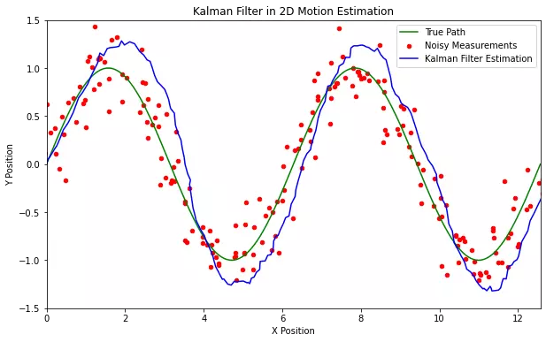
• The green line represents the True Path. This is the actual trajectory of the object. In real-world scenarios, we wouldn't know this unless we had a perfect measuring system (which is typically not the case).
• The red dots represent the Noisy Measurements. These are what our hypothetical sensors (with their inherent inaccuracies) are recording as the object's position.
• The blue dashed line represents the Kalman Filter Estimation. By taking into account both the system's prediction and the noisy measurements, the Kalman filter provides a more accurate and smoother estimate of the object's path.

Why Use the Kalman Filter?

From the visualization, you might be asking, "Why not just use the true path? Why bother with the Kalman filter?" In real-world scenarios, the true path (green line) is unknown to us. We rely on sensors to provide measurements, and these sensors are seldom perfect. They are affected by various sources of noise — from environmental disturbances to electronic noise. The Kalman filter helps us make the best possible estimate of the true state of the system by combining our system model's predictions with sensor measurements.

More Advanced Applications of Kalman Filter with OpenCV

Beyond simple motion tracking, the Kalman filter's predictive capabilities are employed in a variety of advanced computer vision tasks. Some notable applications include:

1. Object Tracking in Videos: In videos, objects can get temporarily occluded. The Kalman filter can predict an object's location during these occlusions, improving tracking robustness.
2. Gesture Recognition: By tracking hand movements, the Kalman filter can contribute to recognizing specific gestures in real-time applications.
3. Robot Navigation: Robots use sensors to navigate their environment. The Kalman filter can help in predicting a robot's position, especially when sensors give conflicting measurements.
4. Structure from Motion (SfM): In 3D reconstruction tasks, the Kalman filter assists in estimating 3D points and camera positions across frames.

Limitations and Considerations

While the Kalman filter is powerful, it's essential to understand its limitations:

1. Linear Assumption: The standard Kalman filter assumes that the system is linear. For non-linear systems, variations like the Extended Kalman Filter (EKF) or the Unscented Kalman Filter (UKF) are used.
2. Noise Characteristics: The filter assumes that the process and measurement noises are Gaussian and white. This might not always be the case in real-world applications.
3. Model Accuracy: The accuracy of the Kalman filter's estimates heavily relies on the accuracy of the system model. If the model is wrong, the Kalman filter's predictions will also be off.

Conclusion and Further Reading

The Kalman filter, with its mathematical elegance and practical utility, has become a cornerstone in the fields of control systems and computer vision. This article provided a foundational understanding of the Kalman filter, demonstrated its implementation in Python using OpenCV, and showcased its application in 2D motion estimation.

For those keen on diving deeper, here are some recommended resources:

1. OpenCV's Documentation on Kalman Filters
2. "Kalman and Bayesian Filters in Python" by Roger R. Labbe Jr.
3. "Optimal State Estimation: Kalman, H Infinity, and Nonlinear Approaches" by Dan Simon.

By understanding the underlying principles and harnessing the power of libraries like OpenCV, one can effectively apply the Kalman filter to various real-world challenges. Whether you're designing a self-navigating robot, developing a gesture-based interface, or venturing into another domain, the Kalman filter is an invaluable tool in your computational arsenal.