Introduction to Wavelet Transform using Python

The world of signal processing is a fascinating blend of mathematics, engineering, and computer science. From audio to images, and even to more abstract concepts like financial time series, the ability to manipulate and analyze signals is crucial. Among the many tools available to the signal processing engineer, the Wavelet Transform stands out due to its flexibility and adaptability. In this article, we'll delve deep into the intuition behind wavelets, show practical examples, and provide insightful visualizations using Python.

What is a Wavelet?

At a fundamental level, a wavelet is a small wave. The term "small" is used to denote that it has limited duration. Unlike sinusoids, which extend from \(-\infty\) to \(+\infty\), wavelets are localized in time, giving them unique properties ideal for certain applications.

Mathematically, a wavelet must satisfy the following condition:

\[
\int_{-\infty}^{\infty} \psi(t) , dt = 0
\]

This means that the wavelet has equal positive and negative areas, resulting in zero mean.

Imagine you're trying to understand a complex musical piece. If you break down the piece by individual instruments, you get a clearer understanding of the composition. The Wavelet Transform does something similar for signals.

The Fourier Transform, another powerful tool, breaks down a signal into its sinusoidal components. However, it lacks time localization. This means, if a brief but significant event occurs in a signal, the Fourier Transform might not capture it effectively.

Enter wavelets. With their localized nature, wavelets can capture both frequency and time information. This dual nature makes them especially suited for non-stationary signals, where the signal's properties change over time.

Continuous Wavelet Transform (CWT)

The CWT allows us to examine a signal at different scales and positions. Mathematically, it's represented as:

\[
CWT_x(a, b) = \int_{-\infty}^{\infty} x(t) \cdot \frac{1}{\sqrt{|a|}} \psi\left(\frac{t - b}{a}\right) , dt,
\]

where:

• \(x(t)\) is the input signal.
• \(\psi\) is the wavelet function.
• \(a\) is the scale factor, giving information about the frequency component.
• \(b\) is the translation factor, providing time localization.

Think of the CWT as a magnifying glass. As you adjust the magnification (scale \(a\)), you can zoom in on specific parts of the signal, and as you move the magnifying glass (translation \(b\)), you can examine different time instances.

Discrete Wavelet Transform (DWT)

While the CWT is continuous in nature, in the digital realm, we often work with discrete signals. The DWT provides a computationally efficient method to analyze signals at various resolutions.

The DWT decomposes a signal into two sets of coefficients: approximation coefficients (\(c_A\)) and detail coefficients (\(c_D\)). This decomposition is achieved using two sets of functions: scaling functions (\(\phi(t)\)) and wavelet functions (\(\psi(t)\)).

Given a discrete signal \(x[n]\), the DWT coefficients at scale \(s\) and position \(l \) are defined as:

• Approximation Coefficients:
  \[
  c_A[s, l] = \sum_{n} x[n] \phi \left( \frac{n - 2^s l}{2^s} \right)
  \]
• Detail Coefficients:
  \[
  c_D[s, l] = \sum_{n} x[n] \psi \left( \frac{n - 2^s l}{2^s} \right),
  \]

here:

• \(s\) is the scale factor. Increasing \(s\) provides a broader, more general view of the signal (lower frequency components).
• \(l\) is the translation factor, which dictates the location in the signal being analyzed.
• The functions \(\phi(t)\) and \(\psi(t)\) are derived from a chosen wavelet (e.g., Daubechies, Haar).

The DWT process can be iteratively applied to the approximation coefficients to achieve multi-level decomposition. At each level, the approximation coefficients are further decomposed into a finer set of approximation and detail coefficients. This hierarchical decomposition allows for a multi-resolution analysis of the signal.

Imagine you are examining a landscape using binoculars. As you adjust the zoom (akin to changing the scale \(s\)), you can focus on broader terrains or zoom in on specific details. The approximation coefficients capture the broader view, while the detail coefficients capture the specific intricacies. By adjusting the position \(l\), you can explore different parts of the landscape. The DWT, through its scales and translations, allows you to explore the "landscape" of a signal in a similar manner.

The Discrete Wavelet Transform provides a flexible framework to analyze signals at various resolutions. By capturing both the broad trends (approximation) and the minute details (details), it offers a comprehensive view of the underlying characteristics of a signal.

Wavelet Transform in Python: Practical Examples

Let's dive into some code. We'll use the PyWavelets (pywt) library in Python to demonstrate the Wavelet Transform.

Setting up the Environment

First, let's import the necessary libraries:

import numpy as np
import matplotlib.pyplot as plt
import pywt

1. Simple Signal Analysis using DWT

Consider a simple signal composed of two sinusoids of different frequencies. We'll use the DWT to analyze this signal.

# Generate the signal
t = np.linspace(0, 1, 1000, endpoint=False)
signal = np.cos(2.0 * np.pi * 7 * t) + np.sin(2.0 * np.pi * 13 * t)

# Apply DWT
coeffs = pywt.dwt(signal, 'db1')
cA, cD = coeffs

# Plotting
plt.figure(figsize=(12, 4))
plt.subplot(1, 3, 1)
plt.plot(t, signal)
plt.title("Original Signal")
plt.subplot(1, 3, 2)
plt.plot(cA)
plt.title("Approximation Coefficients")
plt.subplot(1, 3, 3)
plt.plot(cD)
plt.title("Detail Coefficients")
plt.tight_layout()
plt.show()

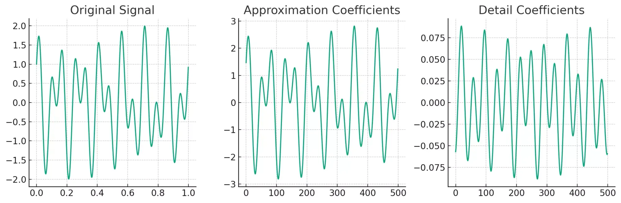
The approximation coefficients capture the general trend of the signal, while the detail coefficients provide insights into the high-frequency components.

• The "Original Signal" plot shows a signal composed of two sinusoids of different frequencies.
• The "Approximation Coefficients" provides a broad overview of the signal, focusing on its low-frequency components.
• The "Detail Coefficients" capture the high-frequency components, allowing us to see the variations and intricacies of the signal.

2. Visualizing Wavelet Transform of a Non-Stationary Signal

Now, consider a signal that has a changing frequency over time. We'll use the CWT for a richer representation.

# Generate a chirp signal
t = np.linspace(0, 1, 1000, endpoint=False)
signal = np.sin(2.0 * np.pi * 7 * t * t)

# Apply CWT
coefficients, frequencies = pywt.cwt(signal, scales=np.arange(1, 128), wavelet='cmor')

# Plotting
plt.figure(figsize=(10, 6))
plt.imshow(np.abs(coefficients), aspect='auto', cmap='jet', extent=[0, 1, 1, 128])
plt.colorbar(label="Magnitude")
plt.ylabel("Scale")
plt.xlabel("Time")
plt.title("CWT of a Chirp Signal")
plt.show()

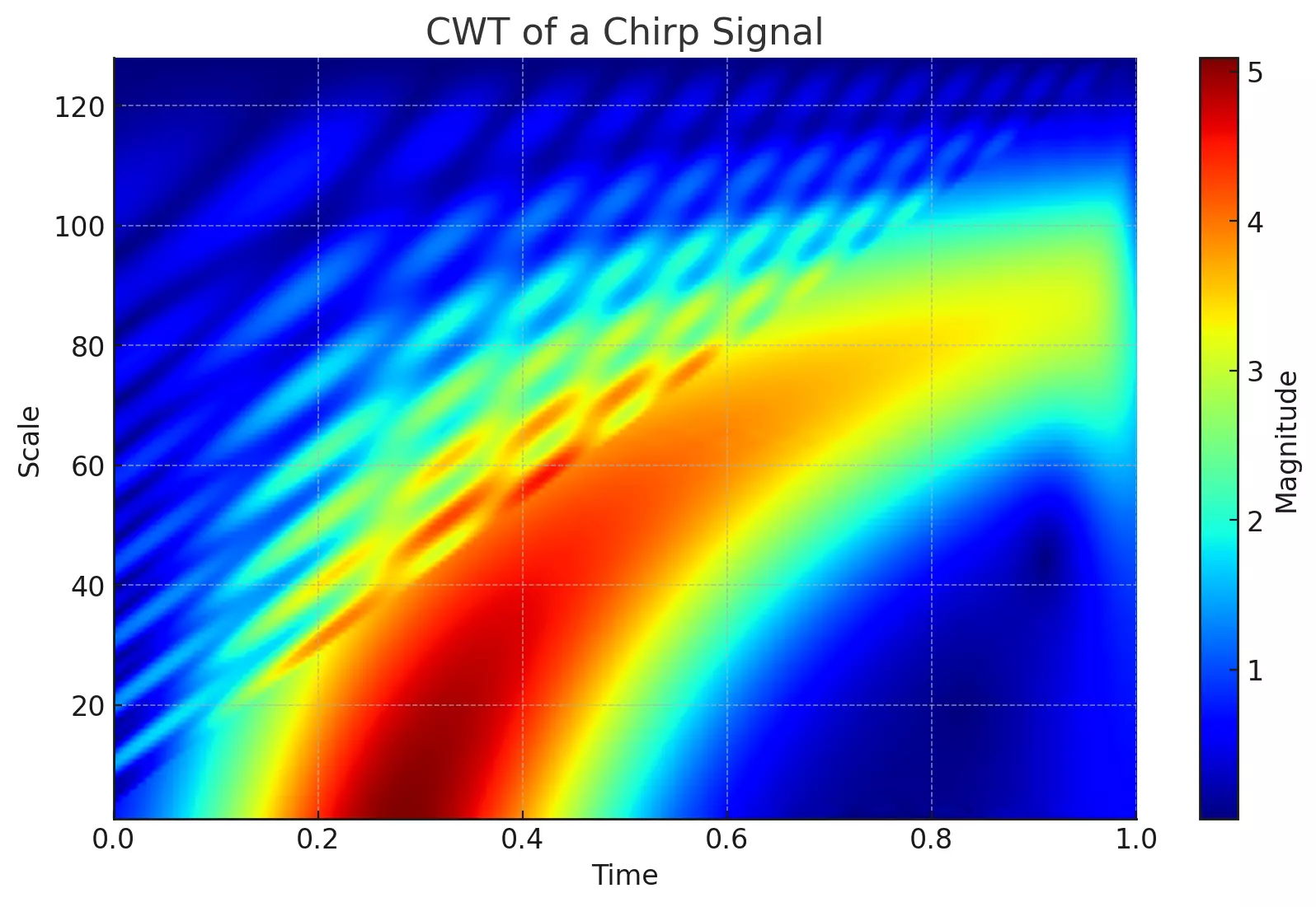
The heatmap from the "CWT of a Chirp Signal" showcases a chirp signal, which has a frequency that changes over time. The color intensity represents the magnitude of the coefficients at different scales (y-axis) and time points (x-axis). Darker shades of blue indicate regions with less energy, while brighter shades (toward yellow) indicate regions with more energy. As can be observed, the frequency of the signal increases as time progresses.

Certainly! Let's explore more practical examples using the Wavelet Transform.

3. Denoising a Signal

One of the primary applications of the Wavelet Transform is denoising signals. Let's take a simple sinusoidal signal, introduce some noise, and then use the wavelet transform to denoise it.

Generate a Noisy Signal

We'll start by generating a simple sinusoidal signal and adding random noise to it.

# Generate a simple sinusoidal signal
t = np.linspace(0, 1, 1000, endpoint=False)
clean_signal = np.sin(2.0 * np.pi * 10 * t)

# Add random noise
noise = np.random.normal(0, 0.5, clean_signal.shape)
noisy_signal = clean_signal + noise

# Plotting the clean and noisy signals
plt.figure(figsize=(12, 4))
plt.subplot(1, 2, 1)
plt.plot(t, clean_signal)
plt.title("Clean Signal")
plt.subplot(1, 2, 2)
plt.plot(t, noisy_signal)
plt.title("Noisy Signal")
plt.tight_layout()
plt.show()

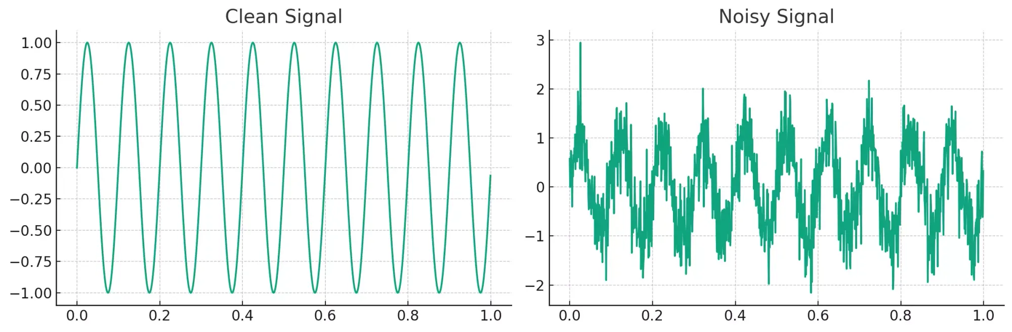
As seen in the plots:

• The "Clean Signal" is a simple sinusoidal wave.
• The "Noisy Signal" has random noise added, which obscures the original waveform.

Denoising Using Wavelet Transform

To denoise the signal, we'll:

1. Decompose the noisy signal using the Discrete Wavelet Transform (DWT).
2. Threshold the detail coefficients to remove the noise.
3. Reconstruct the denoised signal using the Inverse Discrete Wavelet Transform (IDWT).

# Perform a multi-level wavelet decomposition
coeffs = pywt.wavedec(noisy_signal, 'db1', level=4)

# Set a threshold to nullify smaller coefficients (assumed to be noise)
threshold = 0.5
coeffs_thresholded = [pywt.threshold(c, threshold, mode='soft') for c in coeffs]

# Reconstruct the signal from the thresholded coefficients
denoised_signal = pywt.waverec(coeffs_thresholded, 'db1')

# Plotting the noisy and denoised signals
plt.figure(figsize=(12, 4))
plt.subplot(1, 2, 1)
plt.plot(t, noisy_signal)
plt.title("Noisy Signal")
plt.subplot(1, 2, 2)
plt.plot(t, denoised_signal)
plt.title("Denoised Signal")
plt.tight_layout()
plt.show()

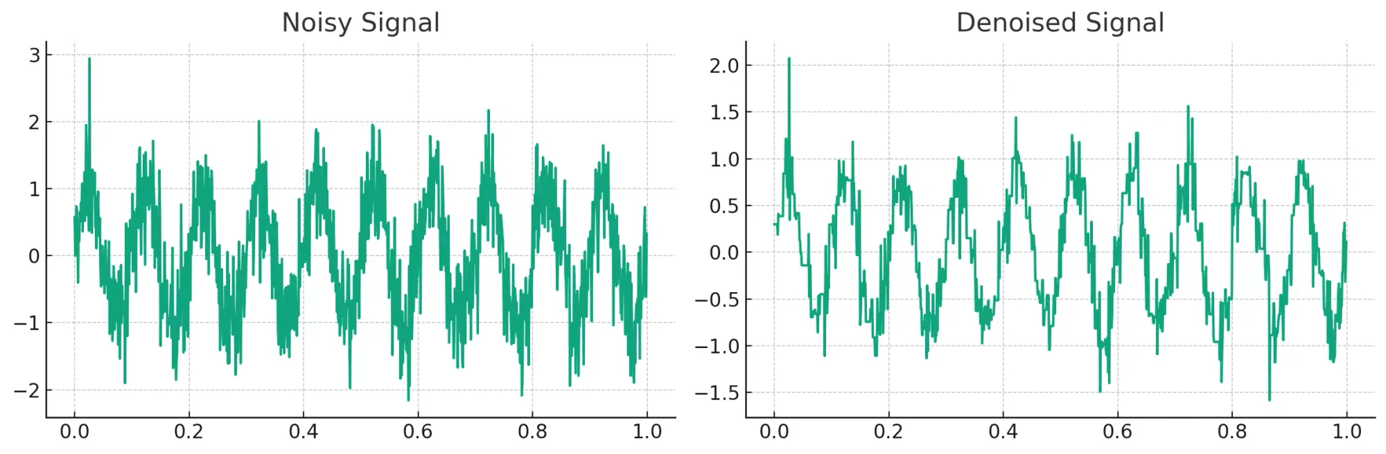
The results clearly demonstrate the efficacy of wavelet-based denoising:

• The "Noisy Signal" plot shows the signal with the introduced random noise.
• The "Denoised Signal" plot presents the result after applying wavelet-based denoising. The waveform closely resembles the original clean signal, with most of the noise removed.

4. Image Compression using Wavelet Transform

Wavelet Transform can also be applied to 2D data, like images, for tasks such as compression. In this example, we'll apply the Discrete Wavelet Transform to an image, threshold the coefficients to retain only the significant ones, and then reconstruct the compressed image.

Generate a Sample Image

We'll create a simple 2D image with varying intensity patterns to demonstrate this.

# Generate a simple 2D image
x, y = np.mgrid[0:1:128j, 0:1:128j]
img = np.sin(2.0 * np.pi * 7 * x) + np.sin(2.0 * np.pi * 13 * y)

# Plotting the generated image
plt.figure(figsize=(5, 5))
plt.imshow(img, cmap='gray')
plt.title("Generated Image")
plt.colorbar()
plt.show()

The generated image is a simple 2D pattern with varying intensities in both the horizontal and vertical directions.

Image Compression using Wavelet Transform

To compress the image:

1. Decompose the image using the Discrete Wavelet Transform (DWT).
2. Threshold the coefficients, keeping only the significant ones.
3. Reconstruct the compressed image using the Inverse Discrete Wavelet Transform (IDWT).

# Flatten and concatenate all the 2D coefficients
all_coeffs = np.concatenate([c.ravel() for sublist in coeffs2 for c in sublist if isinstance(c, np.ndarray)])

# Determine a threshold to retain a certain percentage of the strongest coefficients
percent = 10  # retain only the top 10% of coefficients
threshold = np.percentile(np.abs(all_coeffs), 100 - percent)

# Threshold the coefficients
coeffs2_thresholded = [(pywt.threshold(c, threshold, mode='soft') if isinstance(c, np.ndarray) else c) 
                       for c in coeffs2]

# Reconstruct the compressed image
compressed_img = pywt.waverec2(coeffs2_thresholded, 'db1')

# Plotting the original and compressed images
plt.figure(figsize=(10, 5))
plt.subplot(1, 2, 1)
plt.imshow(img, cmap='gray')
plt.title("Original Image")
plt.colorbar()
plt.subplot(1, 2, 2)
plt.imshow(compressed_img, cmap='gray')
plt.title("Compressed Image")
plt.colorbar()
plt.tight_layout()
plt.show()

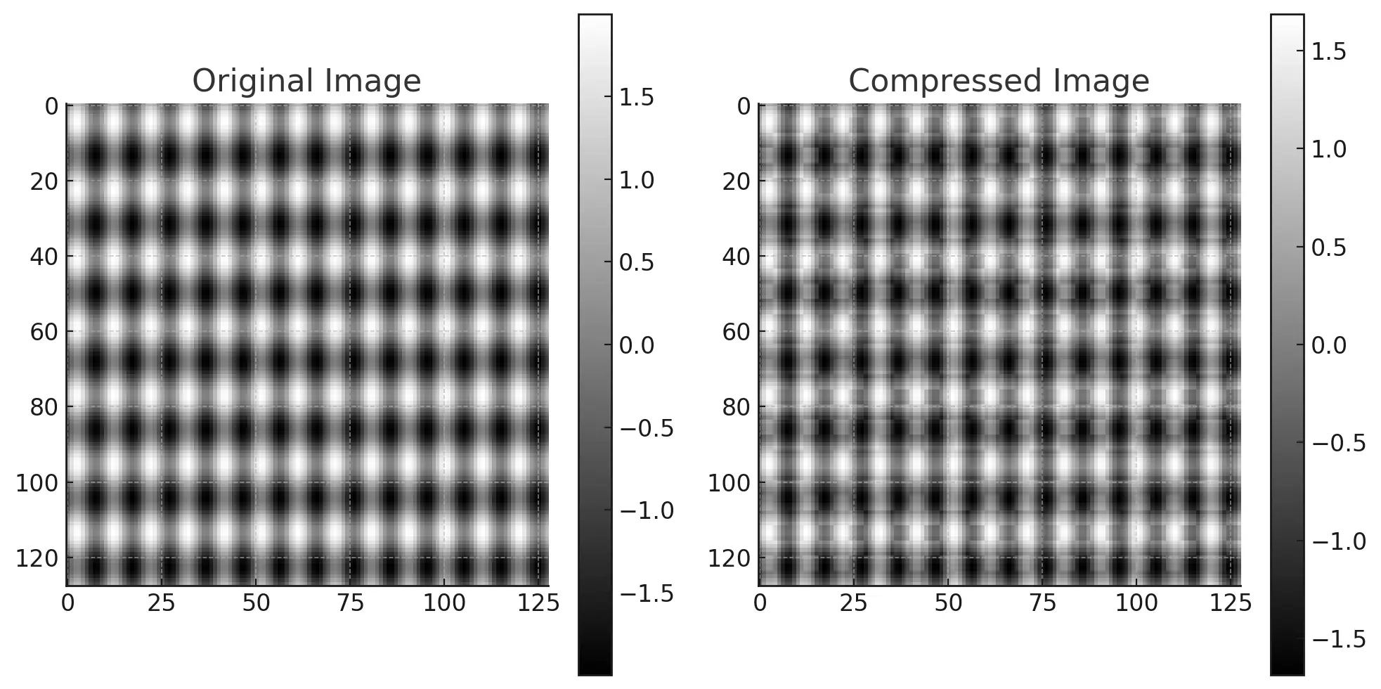
• The "Original Image" showcases the generated pattern.
• The "Compressed Image" is the result after applying wavelet-based compression. We retained only the top 10% of the strongest wavelet coefficients. Despite the significant reduction in coefficients, the compressed image closely resembles the original, demonstrating the efficiency of wavelet-based image compression.

5. Edge Detection in Images using Wavelet Transform

Wavelet Transform can also be used for edge detection in images due to its ability to capture high-frequency changes. We'll use scikit-image library to get a "standard" image for our edge detection tests.

from skimage import data

# Use a built-in image from scikit-image as an example
img_photo = data.camera()

# Plotting the original image
plt.figure(figsize=(5, 5))
plt.imshow(img_photo, cmap='gray')
plt.title("Original Image")
plt.colorbar()
plt.show()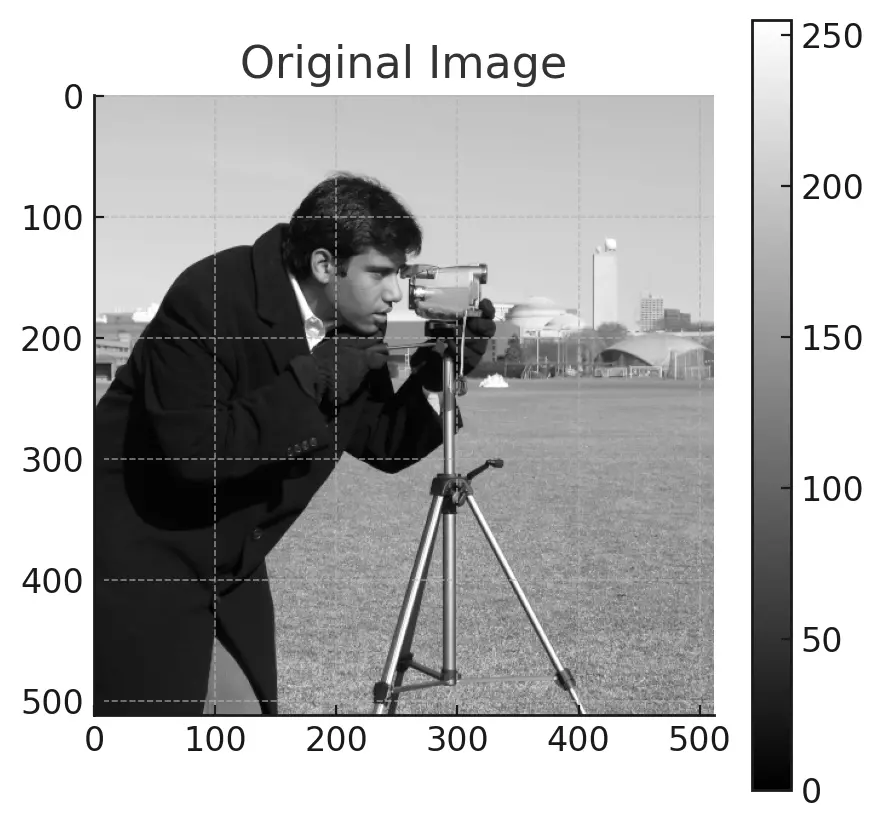

Edge Detection using Wavelet Transform

To detect edges:

1. Decompose the image using the Discrete Wavelet Transform (DWT).
2. The detail coefficients from the decomposition will highlight the high-frequency changes, which correspond to edges in the image.

# Perform a 2D wavelet decomposition on the image
coeffs_photo = pywt.wavedec2(img_photo, 'db1', level=1)
cA_photo, (cH_photo, cV_photo, cD_photo) = coeffs_photo

# Plotting the detail coefficients (edges)
plt.figure(figsize=(15, 5))
plt.subplot(1, 3, 1)
plt.imshow(np.abs(cH_photo), cmap='gray')
plt.title("Horizontal Detail (Edges)")
plt.colorbar()
plt.subplot(1, 3, 2)
plt.imshow(np.abs(cV_photo), cmap='gray')
plt.title("Vertical Detail (Edges)")
plt.colorbar()
plt.subplot(1, 3, 3)
plt.imshow(np.abs(cD_photo), cmap='gray')
plt.title("Diagonal Detail (Edges)")
plt.colorbar()
plt.tight_layout()
plt.show()

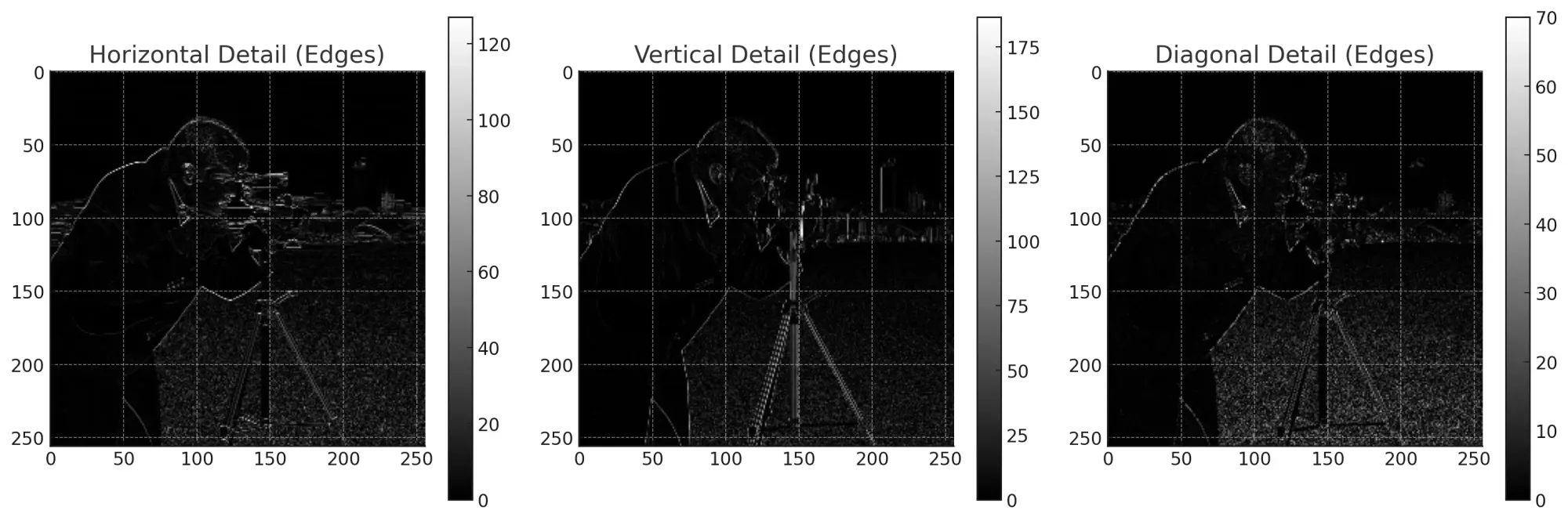
• Horizontal Detail (Edges): Captures edges with horizontal changes. The sharp horizontal transitions in the original image are clearly highlighted here.
• Vertical Detail (Edges): Captures edges with vertical changes. The sharp vertical transitions in the original image are evident in this plot.
• Diagonal Detail (Edges): Captures diagonal features or changes. While our original image didn't have explicit diagonal edges, the interaction of horizontal and vertical edges led to some diagonal details being captured.

This demonstration emphasizes how wavelet decomposition can effectively capture and distinguish various features in an image, making it an invaluable tool for tasks like edge detection.

These practical examples underscore the versatility and power of the Wavelet Transform across various domains, from signal processing to image analysis.

Wrapping Up

The Wavelet Transform, with its dual nature of capturing time and frequency information, is a powerful tool in signal processing. Its adaptability to non-stationary signals gives it an edge in numerous applications, from image compression to denoising audio signals. Python, with libraries like pywt, makes it easier than ever to visualize and understand this transformative technique.

This article offers just a glimpse into the world of wavelets. As with any topic in signal processing, there's much more to explore and understand. Dive deeper, experiment with different signals, and see how wavelets can unveil hidden patterns in your data.