Python

How to do Spectrogram in Python

Learn how to do spectrogram in Python using the essential signal processing packages.

Jake @Scicoding

May 26, 2023 • 8 min read

How to do Spectrogram in Python

In this post, you will learn how to generate a spectrogram in Python. We will utilize the essential Python signal processing packages to find out different ways of calculating the spectrograms.

The spectrogram is a powerful tool for analyzing and visualizing the frequency content of a signal as it changes over time. The fundamental intuition behind a spectrogram is the concept of transforming time-domain data into the frequency domain to uncover additional insights.

In many practical scenarios, it's important not only to know which frequencies are present in a signal but also when these frequencies occur. For example, in music, a piece's melody is not only determined by the specific notes (i.e., frequencies) played, but also by the order and timing of these notes. Similarly, in speech, the meaning of spoken words is determined by the sequence of sounds (phonemes), which are characterized by their specific frequency patterns over time.

The spectrogram provides a two-dimensional representation of a signal, where one axis represents time, the other represents frequency, and the color or intensity represents the magnitude of the signal at each frequency and time. This means you can read the spectrogram as a series of vertical slices, each representing the frequency content of the signal at a specific moment in time.

In effect, a spectrogram is like a series of photographs of the signal's frequency content. Each "photograph" captures the frequency content at a specific moment, and by placing these photographs side by side in time order, you can visualize how the frequency content changes over time. This "time-frequency" representation provides a more comprehensive view of the signal than either the time-domain waveform or the frequency-domain spectrum alone.

Practical applications of spectrogram

Spectrograms are extensively used in various fields, as they provide a way to visualize how the frequencies of a signal are distributed with respect to time. They offer insights into the spectral content of the signal over time, which can be particularly useful in fields such as music and speech processing, seismology, and radio communications, among others.

Music and Speech Processing: Spectrograms are invaluable in music and speech analysis, as they help identify different notes and phonemes based on the frequency content and its changes over time. In music, for example, spectrograms can help visualize the harmonic structure of a piece or detect the rhythm and tempo. In speech processing, they are used in speech recognition systems to identify distinct phonetic features. Further, in voice signal processing, spectrograms can assist in identifying specific voice disorders.

Seismology: In seismology, spectrograms are used to analyze seismic waves generated by earthquakes or volcanic activities. These waves have distinct frequency content that varies over time, providing critical information about the underlying geological processes. Analyzing the spectrogram of these waves allows seismologists to gain insights into the source mechanism of earthquakes or the magma movement inside volcanoes.

Radio Communications: In radio and wireless communication, spectrograms help in analyzing the frequency content of transmitted signals. This can be especially important in identifying interference in the signals or for spectrum management, ensuring that different communication systems don't interfere with each other. They are also used in cognitive radio systems to identify vacant frequency bands dynamically.

Bioacoustics: In the field of bioacoustics, researchers analyze animal sounds using spectrograms. For instance, the study of bird songs, dolphin clicks, or bat echolocation signals. This analysis helps in understanding animal behavior, species identification, and population estimation.

Audio Forensics: Spectrograms are used in audio forensics to analyze recorded audio files. The frequency content can reveal information about the recording environment, and the recording device used, or help to identify tampering in the recorded audio.

These are just a few examples of the practical use cases of spectrograms. They have found applications in an array of disciplines wherever there is a need to understand the frequency behavior of signals over time.

The Mathematical model

The Short-Time Fourier Transform (STFT), and hence the spectrogram, is usually computed using the Fast Fourier Transform (FFT).

Let's consider a discrete signal \(x[n]\), where \(n\) is a discrete-time index. The discrete version of the STFT for a window of length \(N\) centered at time \(m\) and frequency \(k\) can be calculated as follows:

\[
\text{STFT}_{x}[m, k] = \sum_{n=-\infty}^{\infty} x[n]w[n - m]e^{-j2\pi kn/N}
\]

In the equation above, \(w[n - m]\) is the window function, which is typically non-zero for \(n = m - N/2, m - N/2 + 1, ..., m + N/2\) and zero elsewhere.

The FFT is used to efficiently compute the sum in the equation. In particular, for a window of length \(N\), the sum becomes a sum over \(N\) terms, and the FFT can compute all (N) frequency components \(\text{STFT}_{x}[m, k]\) for \(k = 0, 1, ..., N-1\) in \(O(N \log N)\) time, which is much more efficient than the \(O(N^2)\) time it would take to compute each frequency component separately.

Finally, the spectrogram \(S_x[m, k]\) is the square magnitude of the STFT:

\[
S_{x}[m, k] = |\text{STFT}_{x}[m, k]|^{2}
\]

This gives us a 2D representation of how the power of the different frequencies in the signal \(x[n]\) varies with time. Each point in the spectrogram corresponds to a specific time and frequency, and its value corresponds to the power of the signal at that frequency and time.

Creating a spectrogram

A spectrogram is basically a 2D representation where one axis is time, the other is frequency, and the color represents the magnitude of a specific frequency at a specific time. To create a spectrogram, we usually split our signal into smaller chunks or frames (often with some overlap), apply a window function, and then apply the Fourier Transform to each of these frames. This results in a series of spectra, which can be arranged side by side to form the spectrogram.

Test data set

We create a \(10s\) test dataset with a single varying frequency sinusoid. We use \(F_s = 1\text{kHz} = 100\text{Hz}\) sampling frequency.

For the first \(5s\), we use frequency \(F_1 = 10\text{Hz}\) and for the latter \(5s\), we use \(F_2 = 20\text{Hz}\).

The discrete-time test signal is then explicitly defined as
\[ x(n) = \begin{cases}
\sin(2\pi F_1 \frac{n}{F_s}) = 0, \text{ if } \frac{n}{F_s} <= 5s\\
\sin(2\pi F_2 \frac{n}{F_s}) = 0, \text{ if } \frac{n}{F_s} > 5s
\end{cases} \]

where \(n < 5000\).

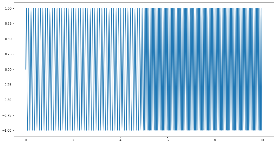
With the spectrogram, we should see the change in frequency at 5s.

import numpy as np
import matplotlib.pyplot as plt

# Define constants
T = 5.0     # seconds
Fs = 100.0 # Sample rate 
N = int(T * Fs) # Total number of samples

F1 = 10.0 # Frequency of signal 1
F2 = 20.0 # Frequency of signal 2

# Create a time array for each segment
t1 = np.linspace(0.0, T, N, endpoint=False)
t2 = np.linspace(T, 2*T, N, endpoint=False)

# Generate sinusoidal signal for each segment
s1 = np.sin(F1 * 2 * np.pi * t1)
s2 = np.sin(F2 * 2 * np.pi * t2)

# Combine the signals and the time arrays
s = np.concatenate([s1, s2])
t = np.concatenate([t1, t2])

SciPy implementation

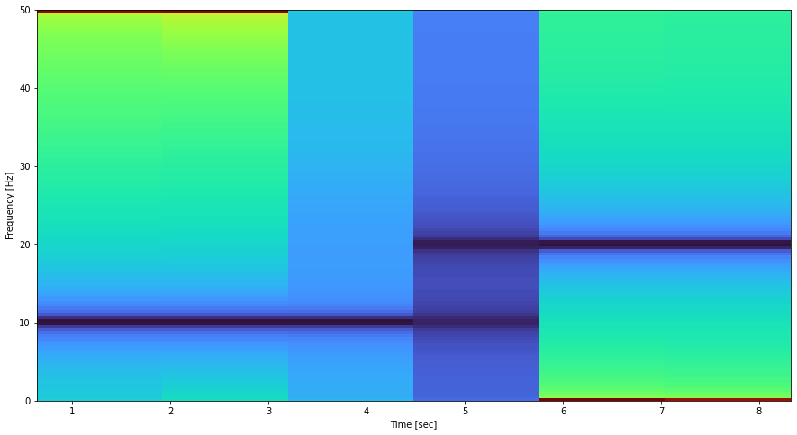
Our go-to package for all signal processing related scipy has readily supported spectrograms.

# SciPy implementation

from scipy import signal
import matplotlib.pyplot as plt

f, t, Sxx = signal.spectrogram(x, Fs)
plt.figure(figsize=(15,8))
plt.pcolormesh(t, f, Sxx, shading='gouraud')
plt.ylabel('Frequency [Hz]')
plt.xlabel('Time [sec]')
plt.ylim([0, 50])
plt.show()

Creating spectrogram using SciPy

Scipy spectrogram produces the following

Plotting spectrogram with Matplotlib

The de-facto plotting package matplotlib also has support for spectrograms. This is convenient, particularly, when all we need is to plot the spectrogram without further analysis.

# Matplotlib plotting of spectrogram

import matplotlib.pyplot as plt

plt.figure(figsize=(15,8))
plt.specgram(s, Fs=Fs, cmap='turbo_r')
plt.ylabel('Frequency [Hz]')
plt.xlabel('Time [sec]')
plt.ylim([0, 50])
plt.show()

Creating spectrogram using Matplotlib

The matplotlib spectrogram produces the following

Numpy only implementation

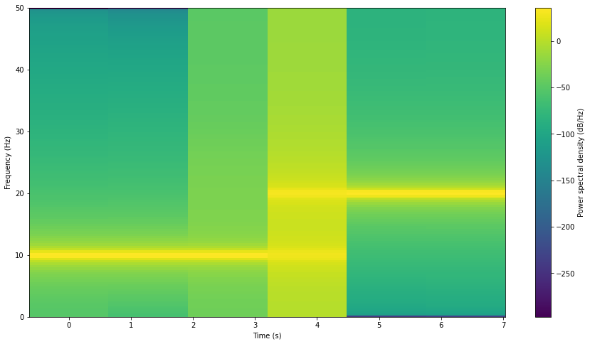
Finally, we consider a NumPy-only implementation, which closely follows the definition of the SFFT. For practical applications, I would recommend not using this implementation as it has not been optimized for performance at all. However, it does serve as a reference on how to build the spectrogram from scratch.

Implementing a spectrogram involves the following steps:

Windowing the signal: The first step is to divide the entire signal into overlapping windows. This is done because the Fourier Transform assumes that the signal is periodic and extends infinitely. For real-world signals, this is not the case, so we use a window function to minimize the effects at the beginning and end of the time window.

Applying the Fourier Transform: The Fourier Transform is then applied to each of these windows to convert them into the frequency domain.

Calculating the power spectrum: The result of the Fourier Transform is a complex number, so we calculate the magnitude of these numbers to get the power of the signal at different frequencies.

Plotting the spectrogram: The spectrogram is plotted as a 2D heatmap, where the x-axis represents time, the y-axis represents frequency, and the color represents the power of the signal.

Here is a basic Python code for creating a spectrogram from scratch using only NumPy and Matplotlib:

import numpy as np
import matplotlib.pyplot as plt

# Define the parameters for the spectrogram
window_size = 256  # Window size for the FFT
overlap    = 128  # Overlap between windows

# Window the signal
window = np.hanning(window_size)
windows = [s[i:i+window_size] * window for i in range(0, len(s)-window_size, window_size-overlap)]

# Compute the FFT for each window
spectrogram = [np.abs(np.fft.rfft(win))**2 for win in windows]

# Transpose the result to have time on the x-axis and frequency on the y-axis
spectrogram = np.array(spectrogram).T

# Plot the spectrogram
frequencies = np.fft.rfftfreq(window_size, d=1.0/Fs)
time = np.arange(len(spectrogram[0])) * (window_size - overlap) / Fs
plt.pcolormesh(time, frequencies, 10 * np.log10(spectrogram))
plt.xlabel("Time (s)")
plt.ylabel("Frequency (Hz)")
plt.colorbar(label="Power spectral density (dB/Hz)")
plt.ylim([0, Fs/2.])
plt.show()

Custom implementation of a Spectrogram

This script implements the basic steps to create a spectrogram. There are many ways this code can be optimized and improved, but this should give you a basic understanding of what is involved in creating a spectrogram from scratch.

Spectrogram from custom Python implementation

Conclusion

Creating and analyzing spectrograms in Python is a multi-step process that combines key principles from digital signal processing and Fourier analysis. We started with constructing a test signal and went through the process of windowing this signal, transforming it to the frequency domain using the Fourier Transform, calculating the power spectrum, and ultimately visualizing the spectrogram with libraries like NumPy and Matplotlib.