Python

Eigenspaces - Theory, Calculation and Applications

Jake @Scicoding

Aug 8, 2023 • 6 min read

Eigenspaces, a fundamental concept in linear algebra, have a wide range of applications in various domains of science and engineering. This article delves deep into the realm of eigenspaces, from their fundamental understanding to practical applications and code examples in Python.

Fundamentals and Intuition

An eigenspace of a matrix (or more generally of a linear transformation) is a subspace of the matrix's (or transformation's) domain and codomain that is invariant under the transformation. It's composed of eigenvectors, which are special vectors that only get scaled when subjected to the transformation, not reoriented.

For a square matrix \(A\) and an eigenvalue \(\lambda\), an eigenspace \(E_\lambda\) is the set of all vectors \(v\) such that \(Av = \lambda v\). This equation states that the action of \(A\) on any vector \(v\) in the eigenspace \(E_\lambda\) merely scales the vector and doesn't change its direction.

The set of all eigenvectors associated with a specific eigenvalue, together with the zero vector, forms a vector space, known as an eigenspace. The reason the zero vector is included is that it satisfies the condition \(Av = \lambda v\) for any \(\lambda\) and is part of every vector space.

Note that the zero vector by itself doesn't provide much information about the nature of the transformation, but it is included in the eigenspace for mathematical completeness, as vector spaces are required to contain the zero vector.

Furthermore, the dimension of an eigenspace associated with an eigenvalue \(\lambda\) (i.e., the number of linearly independent eigenvectors associated with \(\lambda\)) is called the geometric multiplicity of \(\lambda\).

It is important to note that not every linear transformation or matrix has an (non-zero) eigenspace. In some cases, certain properties (like being diagonalizable) ensure the existence of a basis of eigenvectors for the entire vector space, thus providing an eigenspace for each eigenvalue.

Understanding eigenspaces and their properties is crucial in many fields, including physics, computer science, and data analysis, as they often allow for a simplified analysis or optimized calculations.

Imagine a transformation that merely stretches or compresses space without changing the direction of any vectors. The vectors that remain unchanged in direction (though possibly stretched or compressed) after this transformation are the eigenvectors. The amount by which they are stretched or compressed is the eigenvalue.

For instance, consider a rubber sheet with vectors drawn on it. If you were to stretch the sheet in one direction, the vectors that only get elongated (and not rotated) are the eigenvectors. The factor by which they get elongated is the eigenvalue.

Finding and Calculating Eigenspaces

To find an eigenspace, we first need to determine the eigenvalues and eigenvectors of a matrix. The eigenspace associated with a specific eigenvalue is the set of all vectors that, when the matrix transformation is applied, are scaled by that eigenvalue, i.e., all vectors that satisfy the equation \(Av = \lambda v\).

Step 1: Find Eigenvalues

The first step is to find the eigenvalues of the matrix. The eigenvalues are the roots of the characteristic equation, which is given by \(|A - \lambda I| = 0\). Here, \(A\) is the given matrix, \(I\) is the identity matrix of the same size as \(A\), and \(\lambda\) represents the eigenvalues.

Solving this equation gives the eigenvalues of \(A\).

Step 2: Find Eigenvectors

Next, we find the eigenvectors associated with each eigenvalue. To do this, we substitute each eigenvalue into the equation \((A - \lambda I)v = 0\), where \(v\) is the vector we are trying to find. This equation represents a system of linear equations.

Step 3: Solve for the Eigenspace

An eigenspace associated with a given eigenvalue is formed by all the eigenvectors associated with that eigenvalue, including the zero vector.

To find the eigenspace for a given eigenvalue, we need to find all solutions to the equation \((A - \lambda I)v = 0\), i.e., we need to solve this system of equations for \(v\). The system will generally have an infinite number of solutions, which form a subspace of the original vector space—the eigenspace.

The process for solving the system of equations generally involves Gaussian elimination or similar methods. The resulting solution set may be parametrized with free variables, which is where the infinite number of solutions arises from.

Finding the Basis of an Eigenspace

The basis of an eigenspace is the set of linearly independent eigenvectors within that eigenspace. Once we've found the general solution to \(A - \lambda I)v = 0\(, the vectors corresponding to the free variables in the solution form a basis for the eigenspace. Each of these basis vectors is an eigenvector corresponding to the eigenvalue we're considering, and together they span the eigenspace. Note that the zero vector, though part of the eigenspace, is not included in the basis since basis vectors must be linearly independent.

The geometric multiplicity of an eigenvalue (the dimension of its eigenspace) is given by the number of linearly independent solutions to \((A - \lambda I)v = 0\), i.e., the number of basis vectors in the eigenspace.

Remember that all these solutions, eigenvectors, are associated with a specific eigenvalue. When you repeat this process for all eigenvalues of your matrix, you effectively decompose your original space into these invariant subspaces, i.e., the eigenspaces.

Applications of Eigenspaces

Eigenspaces have numerous applications across various domains:

Principal Component Analysis (PCA): Used in data science and machine learning, PCA is a technique to reduce the dimensionality of data. Eigenspaces play a crucial role in identifying the directions (principal components) that capture the most variance in the data.

Quantum Mechanics: In quantum physics, eigenstates and eigenvalues play a central role in describing the possible states and measurable quantities of quantum systems.

Differential Equations: Eigenspaces are key to solving systems of linear differential equations, especially in problems like the vibration of systems, heat conduction, and more.

PageRank Algorithm: Used by Google's search engine, the PageRank algorithm relies on eigenvectors and eigenvalues to determine the importance of web pages.

Facial Recognition: Eigenfaces are a set of eigenvectors used in the computer vision problem of human face recognition.

Stability Analysis: In control theory and dynamical systems, the eigenvalues of a system matrix determine the stability of the system.

Code Examples in Python

Let's implement some Python code to determine the eigenspaces of a matrix using the popular numpy library.

Finding Eigenvalues and Eigenvectors

Here's a Python code example on how to find eigenvalues and eigenvectors

import numpy as np

# Define a sample matrix
A = np.array([[4, -2],
              [1,  1]])

# Calculate eigenvalues and eigenvectors
eigenvalues, eigenvectors = np.linalg.eig(A)

eigenvalues, eigenvectors

This gives us

(array([3., 2.]),
 array([[0.89442719, 0.70710678],
        [0.4472136 , 0.70710678]]))

For the sample matrix

\[
A = \begin{bmatrix}
4 & -2 \
1 & 1
\end{bmatrix}
\]

The eigenvalues are \(\lambda_1 = 3\) and \(\lambda_2 = 2\).

The eigenvector corresponding to \(\lambda_1\) is approximately

\[
\begin{bmatrix}
0.8944 \
0.4472
\end{bmatrix}
\]

and for \(\lambda_2\) is approximately

\[
\begin{bmatrix}
0.7071 \
0.7071
\end{bmatrix}
\]

Eigenspace Visualization

To gain a better intuition, let's visualize the eigenspace of a 2x2 matrix. We'll plot the transformation of a grid of vectors by the matrix and highlight the eigenvectors.

We can utilize matplotlib to visualize the eigenspace

import matplotlib.pyplot as plt

def plot_vectors(vectors, colors):
    plt.figure(figsize=(5,5))
    plt.axvline(x=0, color='grey', lw=1)
    plt.axhline(y=0, color='grey', lw=1)
    for i in range(len(vectors)):
        plt.quiver(0, 0, vectors[i][0], vectors[i][1], angles='xy', scale_units='xy', scale=1, color=colors[i])

# Original grid
x = np.linspace(-2, 2, 5)
y = np.linspace(-2, 2, 5)
grid = np.array([[xi, yi] for xi in x for yi in y])

# Transformed grid
transformed_grid = np.dot(A, grid.T).T

# Plotting
plot_vectors(grid, ['blue']*len(grid))
plot_vectors(transformed_grid, ['red']*len(grid))

# Highlighting eigenvectors
plot_vectors(eigenvectors.T, ['green', 'purple'])
plt.xlim(-3, 3)
plt.ylim(-3, 3)
plt.title('Eigenspace Visualization')
plt.show()

In the visualization above:

The blue vectors represent the original grid of vectors.

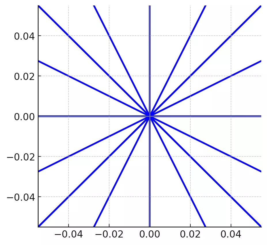
The red vectors depict the transformed grid after being multiplied by matrix \(A\).

The green and purple vectors are the eigenvectors of matrix \(A\).

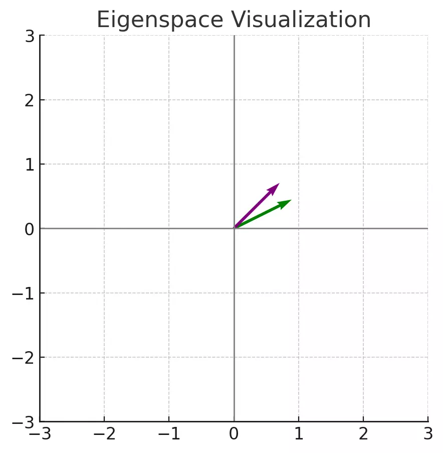
Notice that the eigenvectors (in green and purple) are merely stretched by the matrix transformation and maintain their original directions. This visualization reinforces the concept that eigenvectors are vectors that remain unchanged in direction (though possibly scaled) by the transformation represented by the matrix.

Wrapping Up

Eigenspaces offer a profound insight into the behavior of linear transformations. From data analysis to quantum mechanics, the principles of eigenspaces find applications in myriad domains. With a solid understanding of the underlying concepts and the computational tools provided by languages like Python, one can harness the power of eigenspaces to solve complex problems in science, engineering, and beyond.