Calculating Power Spectral Density in Python
How to calculate power spectral density (PSD) in Python using the essential signal processing packages.

Power spectral density (PSD) shows how the power of a signal is distributed over frequencies. It has applications in signal processing for many engineering disciplines.
Communications systems, such as radios and radars, use PSD to identify the channel occupancy and the related frequencies. Spectrum analysis often utilizes PSD to identify the signal power distribution over a frequency range.
Periodograms are a particular version of PSDs applied for discrete-time signals. As this is the case usually in signal processing for digital systems, we also focus mainly on periodograms in this post.
In the following, we briefly walk through the definition of PSD and periodogram. Then, we will see how PSD is calculated using the essential python signal processing packages scipy and matplotlib. We also show you how to make your own PSD implementation following directly from the mathematical definition.
Power spectral density
We dive straight into the discrete-time signals and skip the whole top-down story starting from continuous signals. Our data is usually sampled, so discrete-time processing is the one that we use in practice.
Let's consider a discrete signal \(\mathbf{x} = (x_1, \ldots, x_N)\), where \(N\) is the length of the signal. This can be either the complete signal or a \(N\)-length window of a bigger signal.
Furthermore, let's assume that the signal is sampled at frequency \(F = {1 \over \Delta t} \), where \(\Delta t\) is the sample interval in seconds.
The total signal or window duration is given by \(T = (N - 1)\Delta t\).
This leads us to the definition of discrete-time power spectral density at frequency \(f\)
\[ \bar{S}_{xx}(f) = \lim_{N \to \infty} {(\Delta t)^2 \over T} \left| \sum_{n = 1}^N x_n e^{-i2fn \Delta t} \right|^2 \]
Note that the theoretical PSD assumes that the signal length approaches infinity. This is of course not the case in real life. Thus, in practice, we consider finite \(N\). Whatever, length is applicable to your scenario. Strictly speaking, this is not PSD but rather a periodogram, which converges to the actual PSD as \(N \to \infty\).
Taking into account the finite signal length, in practice, we consider PSD via periodogram as
\[ S_{xx}(f) = {(\Delta t)^2 \over T} \left| \sum_{n = 1}^N x_n e^{-i2fn \Delta t} \right|^2 \]
We will also follow this formulation when we implement the periodogram calculation using only numpy.
Python solution for PSD
Test data
Before going into calculating the actual PSD, we need to generate some test data. For this purpose, we use two sine waves at frequencies 10Hz and 60Hz. We also throw in some Gaussian noise to see, whether we can find these two frequency components from the signal.
fs = 1000.0 # 1 kHz sampling frequency
F1 = 10 # First signal component at 10 Hz
F2 = 60 # Second signal component at 60 Hz
T = 10 # 10s signal length
N0 = -10 # Noise level (dB)import numpy as np
t = np.r_[0:T:(1/fs)] # Sample times
# Two Sine signal components at frequencies F1 and F2.
signal = np.sin(2 * F1 * np.pi * t) + np.sin(2 * F2 * np.pi * t)
# White noise with power N0
signal += np.random.randn(len(signal)) * 10**(N0/20.0) Using Scipy
The go-to signal analytics package scipy has an implementation for calculating periodograms readily available scipy.signal.periodogram. Using this, we can easily calculate power spectral density. Using Scipy is simple, all we need to give the periodogram method are the actual signal data and sampling frequency. To be sure, we also set scaling='density' to make the method return PSD instead of the power spectrum.
import scipy.signal

# f contains the frequency components
# S is the PSD
(f, S) = scipy.signal.periodogram(signal, fs, scaling='density')
What we get out of the method are the frequency components and the corresponding power density.
Now, we are ready to plot the data.
import matplotlib.pyplot as plt

plt.semilogy(f, S)
plt.ylim([1e-7, 1e2])
plt.xlim([0,100])
plt.xlabel('frequency [Hz]')
plt.ylabel('PSD [V**2/Hz]')
plt.show()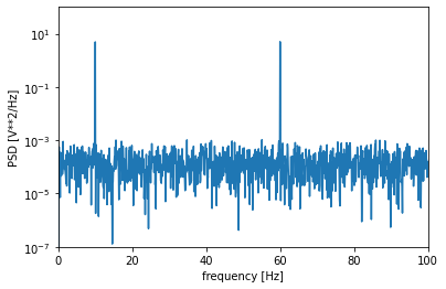
We can quickly identify the two frequency components at their corresponding frequencies: 10Hz & 60Hz. Both have the same amplitude, which makes sense as the sine waves have the same amplitudes.
Estimating PSD using Scipy & Welch's method
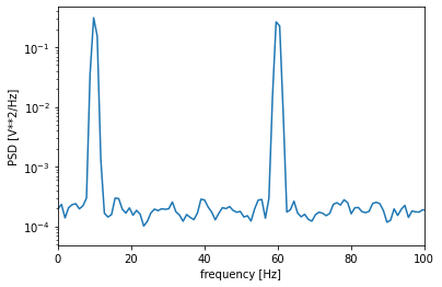
PSD can be somewhat heavy to calculate for long signals. Welch's method is one well-known method to estimate the PSD. Scipy also has a method readily available for using this estimation approach.
(f, S)= scipy.signal.welch(signal, fs, nperseg=1024)

plt.semilogy(f, S)
plt.xlim([0, 100])
plt.xlabel('frequency [Hz]')
plt.ylabel('PSD [V**2/Hz]')
plt.show()
As you can see Welch's method offers a fairly good estimate of the amplitudes and frequency components for our test signal. We can clearly identify the correct frequency components from the noise.
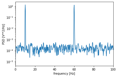
By increasing the segment length, we can get a more accurate estimate.
(f, S)= scipy.signal.welch(signal, fs, nperseg=4*1024)

plt.semilogy(f, S)
plt.xlim([0, 100])
plt.xlabel('frequency [Hz]')
plt.ylabel('PSD [V**2/Hz]')
plt.show()
Using a longer segment length makes the frequency components more distinguishable. This is helpful when there are signal components that are close to each other.
Using Matplotlib
Matplotlib also provides a method for computing and plotting PSD. It uses the aforementioned Welch's method to compute the PSD.
# Matplotlib
import matplotlib.pyplot as plt

(S, f) = plt.psd(signal, Fs=fs)

plt.semilogy(f, S)
plt.xlim([0, 100])
plt.xlabel('frequency [Hz]')
plt.ylabel('PSD [V**2/Hz]')
plt.show()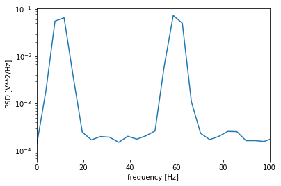
The results are similar to Welch's method using Scipy. If you want to avoid Scipy dependency using Matplotlib can be handy.
Naive Python implementation
We can implement a naive Python implementation with numpy only dependency. This implementation directly follows the definition. It is very slow. But if you only need to calculate PSD for a few frequencies, it might be helpful.
import numpy as np

# f is the requested frequency
# signal is the time series data
# Fs is the sampling frequency in Hz
def Sxx(f, signal, Fs):
    t = 1/Fs # Sample spacing
    T = len(signal) # Signal duration

    s = np.sum([signal[i] * np.exp(-1j*2*np.pi*f*i*t) for i in range(T)])

    return t**2 / T * np.abs(s)**2
Then, to calculate PSD for frequencies \([0, \ldots, 100]\), we can just use
# Use Sxx to calculate PSD for f in [0, 100]
S = [Sxx(f, signal, fs) for f in range(100)]

plt.semilogy([f for f in range(100)], S)
plt.xlim([0, 100])
plt.xlabel('frequency [Hz]')
plt.ylabel('PSD [V**2/Hz]')
plt.show()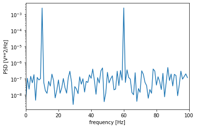
Summary
You have now the essential tools for the calculation of PSDs and periodograms. It is easy with conventional signal processing packages. You should also have an idea of how to implement the PSD method by yourself strictly following the mathematical definition.
Further reading
- Lomb-Scargle periodogram essentially provides PSD for unevenly spaced data
- Principles of Random Signal Analysis and Low Noise Design: The Power Spectral Density and its Applications
- Scipy periodogram documentation
- Scipy Welch's method documentation
- Matplotlib PSD documentation