Python and PCA: Four Techniques to Reduce Dimensions

Principal Component Analysis (PCA) is a dimensionality reduction technique that's widely used in machine learning and statistics. It works by finding a new set of dimensions (or "principal components") that capture the most variance in the data. By reducing the dimensionality of the data, PCA can make data visualization easier, reduce the amount of memory and storage needed, and even improve the performance of some machine learning algorithms.

In this article, we will explore four different ways to perform PCA in Python:

1. Using the scikit-learn library.
2. Using the pandas library.
3. Using the numpy library.
4. Pure Python implementation.

Each approach has its advantages and trade-offs. We'll go through each method step-by-step, providing code examples, visualizations, and intuitive explanations.

Let's start with the first method.

1. PCA Using scikit-learn

Scikit-learn is one of the most popular machine learning libraries in Python. It provides simple and efficient tools for data mining and data analysis. For more in-depth description check our article on how to do PCA using scikit-learn.

Installation:

If you haven't installed scikit-learn yet, you can do so with:

pip install scikit-learn

Implementation:

Let's start by generating some sample data to work with.

import numpy as np
import matplotlib.pyplot as plt

# Generate random data
np.random.seed(0)
X = np.dot(np.random.random(size=(2, 2)), np.random.normal(size=(2, 200))).T

plt.scatter(X[:, 0], X[:, 1], alpha=0.5)
plt.xlabel('x')
plt.ylabel('y')
plt.title('Original Data')
plt.show()

This will give us a scatter plot of our data points. Now, let's apply PCA using scikit-learn.

from sklearn.decomposition import PCA

pca = PCA(n_components=2)
pca.fit(X)

# Transform the data
X_pca = pca.transform(X)

# Visualize the transformed data
plt.scatter(X_pca[:, 0], X_pca[:, 1], alpha=0.5)
plt.xlabel('Principal Component 1')
plt.ylabel('Principal Component 2')
plt.title('Data after PCA')
plt.show()

The transformed data now lies along the principal components, which are the directions of maximum variance.

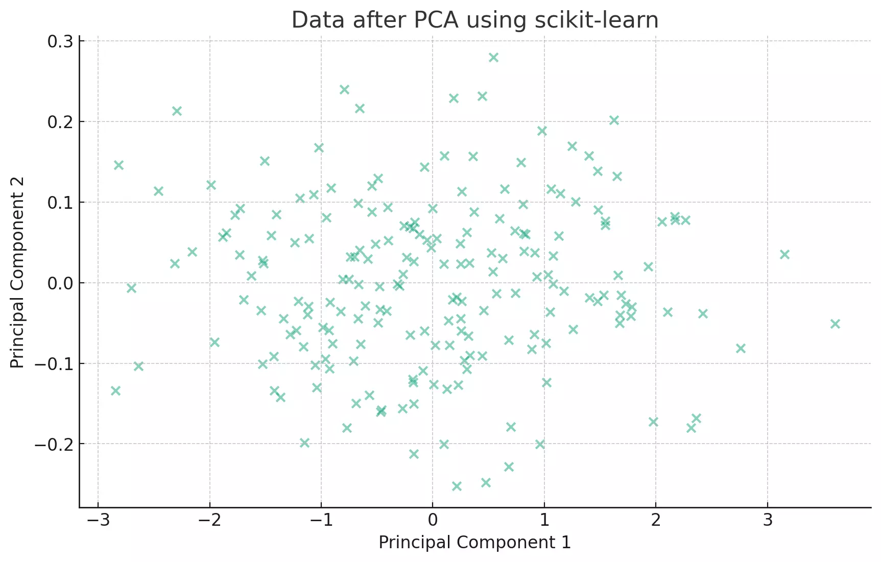
PCA tries to find the axes with maximum variance. In the context of our scatter plot, it's like trying to fit an ellipse to our data points and then finding the major and minor axes of this ellipse.

2. PCA Using pandas

Pandas is a fast, powerful, flexible, and easy-to-use open-source data analysis and data manipulation library built on top of the Python programming language.

Installation:

If you haven't installed pandas yet, you can do so with:

pip install pandas

Implementation:

First, let's create a DataFrame using our sample data from above.

import pandas as pd

df = pd.DataFrame(data=X, columns=["x", "y"])

PCA can be achieved in pandas through its covariance functionality and numpy's linear algebra functions.

# Calculate the covariance matrix
cov_matrix = df.cov()

# Get the eigenvalues and eigenvectors
eigen_values, eigen_vectors = np.linalg.eig(cov_matrix)

# Sort the eigenvectors by decreasing eigenvalues
sorted_index = np.argsort(eigen_values)[::-1]
sorted_eigenvalue = eigen_values[sorted_index]
sorted_eigenvectors = eigen_vectors[:, sorted_index]

# Transform the data
X_pandas = np.dot(X, sorted_eigenvectors)

# Visualize the transformed data
plt.scatter(X_pandas[:, 0], X_pandas[:, 1], alpha=0.5)
plt.xlabel('Principal Component 1')
plt.ylabel('Principal Component 2')
plt.title('Data after PCA using pandas')
plt.show()

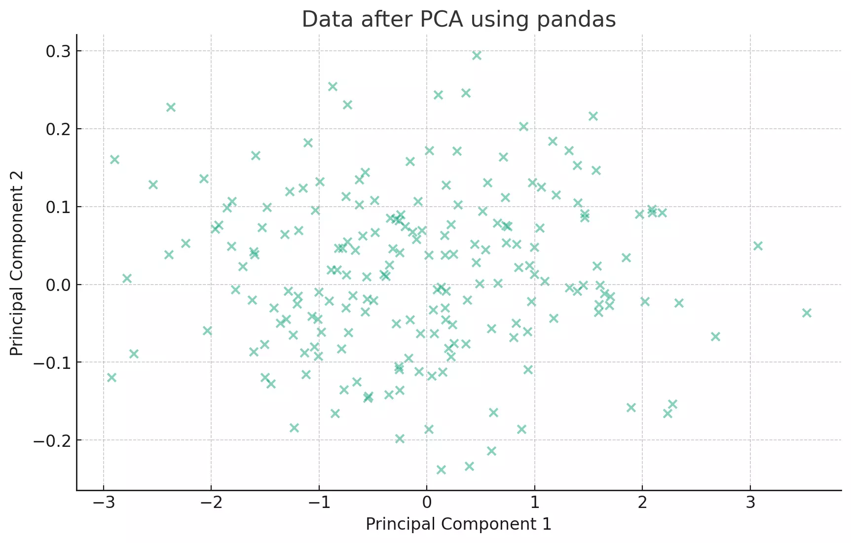
The eigenvectors of the covariance matrix represent the directions of the axes where there is the most variance (i.e., the spread of the data). The eigenvalues represent the magnitude of this variance. By sorting the eigenvectors by the eigenvalues in decreasing order, we get the principal components in order of significance.

3. PCA Using numpy

Numpy is the core library for scientific computing in Python. It provides a high-performance multidimensional array object and tools for working with these arrays.

Implementation:

Since we've already used numpy in the previous examples, we'll just dive into the PCA implementation.

# Compute the mean of the data
mean = np.mean(X, axis=0)

# Center the data by subtracting the mean
centered_data = X - mean

# Compute the covariance matrix
cov_matrix = np.cov(centered_data, rowvar=False)

# Get the eigenvalues and eigenvectors
eigen_values, eigen_vectors = np.linalg.eig(cov_matrix)

# Sort the eigenvectors by decreasing eigenvalues
sorted_index = np.argsort(eigen_values)[::-1]
sorted_eigenvalue = eigen_values[sorted_index]
sorted_eigenvectors = eigen_vectors[:, sorted_index]

# Transform the data
X_numpy = np.dot(centered_data, sorted_eigenvectors)

# Visualize the transformed data
plt.scatter(X_numpy[:, 0], X_numpy[:, 1], alpha=0.5)
plt.xlabel('Principal Component 1')
plt.ylabel('Principal Component 2')
plt.title('Data after PCA using numpy')
plt.show()

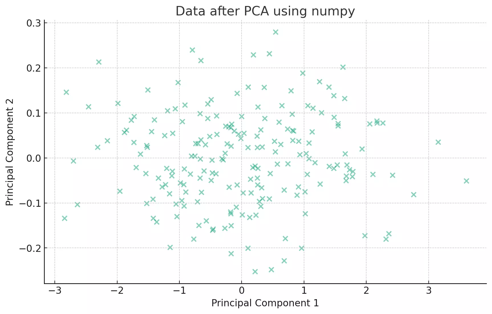
This approach is quite similar to the pandas method. The core difference is in the underlying data structures (numpy arrays vs. pandas DataFrames) and the way the covariance matrix is computed. But the essence, finding the eigenvectors and eigenvalues of the covariance matrix, remains the same.

4. Pure Python Implementation:

This method is a manual, pure Python approach without relying on any external libraries (except for matplotlib for visualization). It serves as a great exercise to understand the underlying mathematics and operations involved in PCA.

1. We will compute the mean of the data and center the data by subtracting the mean.
2. We'll compute the covariance matrix of the centered data.
3. We'll compute the eigenvalues and eigenvectors of the covariance matrix.
4. We'll sort the eigenvectors based on the eigenvalues in decreasing order.
5. Finally, we'll project the centered data onto the sorted eigenvectors to get the principal components.

Given the complexity of eigen decomposition in pure Python, we'll use the power iteration method to approximate the dominant eigenvector and eigenvalue, and then deflate the covariance matrix to get the subsequent eigenvectors and eigenvalues.

Implementation:

Let's start by defining some helper functions.

def transpose(matrix):
    """Return the transpose of a matrix."""
    return [list(row) for row in zip(*matrix)]

def matrix_multiply(A, B):
    """Multiply matrices A and B."""
    return [[dot_product(row, col) for col in transpose(B)] for row in A]

def power_iteration(matrix, num_iterations=1000):
    """Power iteration to find dominant eigenvector and eigenvalue."""
    n, d = len(matrix), len(matrix[0])
    vec = [1] * d
    for _ in range(num_iterations):
        # Multiply matrix by vector
        vec = [dot_product(row, vec) for row in matrix]
        norm = (sum(x**2 for x in vec))**0.5
        vec = [x/norm for x in vec]
    eigenvalue = dot_product(vec, [dot_product(row, vec) for row in matrix])
    return eigenvalue, vec

def deflate(matrix, eigenvalue, eigenvector):
    """Deflate the matrix to find next eigenvector and eigenvalue."""
    n = len(matrix)
    w = [[eigenvalue * eigenvector[i] * eigenvector[j] for j in range(n)] for i in range(n)]
    return [[matrix[i][j] - w[i][j] for j in range(n)] for i in range(n)]

def vector_mean_python(vectors):
    """Compute the mean of vectors in pure Python."""
    num_elements = len(vectors[0])
    return [sum(vector[i] for vector in vectors) / len(vectors) for i in range(num_elements)]

def covariance_python(x, y):
    """Compute covariance in pure Python."""
    n = len(x)
    mean_x = sum(x) / n
    mean_y = sum(y) / n
    return sum((x[i] - mean_x) * (y[i] - mean_y) for i in range(n)) / (n - 1)

def covariance_matrix_python(data):
    """Compute covariance matrix in pure Python."""
    return [[covariance_python(col1, col2) for col1 in zip(*data)] for col2 in zip(*data)]

Now, we are ready to calculate the PCA

# Compute covariance matrix using pure Python functions
cov_matrix_python = covariance_matrix_python(centered_data_final_python)

# Extract eigenvalues and eigenvectors using power iteration and matrix deflation
eigenvalues_python, eigenvectors_python = [], []
for _ in range(2):  # since our data is 2D, we have 2 eigenvectors and eigenvalues
    eigenvalue, eigenvector = power_iteration(cov_matrix_python)
    eigenvalues_python.append(eigenvalue)
    eigenvectors_python.append(eigenvector)
    cov_matrix_python = deflate(cov_matrix_python, eigenvalue, eigenvector)

# Project data onto the eigenvectors
projected_data_python = matrix_multiply(centered_data_final_python, transpose(eigenvectors_python))

# Extract x and y values for visualization
x_vals_python, y_vals_python = zip(*projected_data_python)

# Visualize the result
plt.scatter(x_vals_python, y_vals_python, alpha=0.5)
plt.xlabel('Principal Component 1')
plt.ylabel('Principal Component 2')
plt.title('Data after PCA using pure Python')
plt.show()

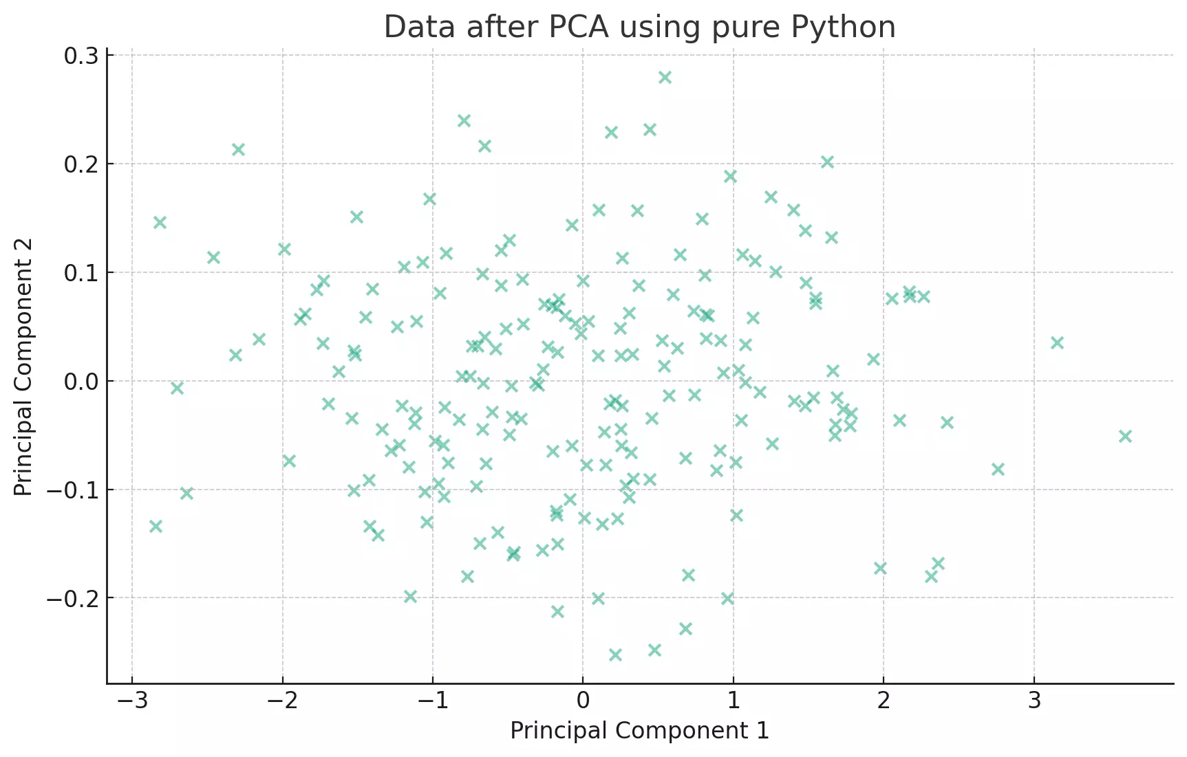
The scatter plot visualizes the data after PCA using a pure Python implementation. The data has been transformed into the axes that represent the most variance. This visualization is consistent with the previous PCA results obtained using other methods.

In summary

1. Scikit-learn: A straightforward method using a machine learning library.
2. Pandas: A data analysis library approach involving eigen decomposition.
3. Numpy: A numerical computation approach focusing on matrix operations.
4. Pure Python: A foundational approach using basic Python functionalities, shedding light on the underlying math.

Each approach offers a unique perspective, with some being more efficient and others more illustrative. The choice of method often depends on the context and the specific requirements of a task.